A Slow but Symmetric FIR Filter Implementation

It’s been some time since we’ve discussed digital filtering on the ZipCPU blog. When we last left the topic, we had several filters left to present. Today, let’s pick up the symmetric or linear phase filter, and demonstrate a block RAM based implementation of it. I’ll call this a slow filter, similar to our last slow filter, simply because this filter won’t be able to handle a new sample every clock tick. Instead, what makes this filter special is that it only requires one dedicated hardware multiply. Better yet, as with the last slow filter implementation, making this filter adjustable won’t require a lot of resources. Unlike the last filter, though, this one will offer nearly twice the performance for nearly the same amount of resources.

Interested yet?

But we’ll come back to this in a moment. In the meantime, let’s try to catch up some of our readers who may be starting in the middle of this discussion. Basically, we’ve been slowly working through hardware implementations of all of the basic FIR filtering types. We’ve already laid a lot of ground work, ground work you might wish to review should you find yourself coming in the middle of this discussion.

Our first post on the topic outlined what a digital filter was, and how a filter could be built that operated at the full clock rate of an FPGA. This initial post was quickly followed by an updated implementation that used fewer flip-flops while achieving the same performance.
This initial filtering article was followed by a proposed abstraction that could be applied to every filtering implementation. As long as any filter we built, therefore, had the I/O interface of this generic filter, we could re-use a test harness, to test multiple different filters.

A following article discussed how we could use this generic filter testing approach to verify that a given filter had the frequency response it was designed to have.

We then demonstrated how these methods could be applied to test our generic FIR filter.
Along the way, we’ve presented several different types of filters. We started by discussing two of the absolute simplest filters I know of: a pairwise averager and a recursive averager.
We then came back later to make the pairwise averager into a more generic moving (block) average filter.
The last post on this topic broke the mold of a filter that accepted one input and produced one output on every clock tick. Instead, that post presented a filter that would accept one input every N clocks, allowing the filter to accomplish all of its multiplies using a single hardware multiply alone.

Further, since this filtering implementation used block RAM to store and retrieve its coefficients, it cost much less to reconfigure the filter than our prior generic filtering implementation.
Since this last post, I’ve focused on interpolation for a while, by first proving that interpolation is a convolution, and then showing how that knowledge could be used to create a very useful quadratic interpolation method with some amazing out-of-band performance.

In other words, it’s been some time since we’ve discussed filtering, and there remain many types of filters and filtering implementations for us still to discuss. For example, we haven’t discussed symmetric or half-band filters. Neither have we discussed how to implement a Hilbert transform. Another fun filtering topic we could discuss would be how to string multiple filters together to handle the case where there may be N clocks between samples, but the filter has more than N coefficients. There’s also the ultimate lowpass filter: the one that filters an incoming sample stream to (just about) any arbitrary low-bandwidth for only about 24 taps–independent of the actual lowpass bandwidth. Then there’s the adaptive filters that are commonly used in the equalizers within digital communications receivers. Finally, there’s the grandaddy filter of them all: the FFT based filter. When implemented properly, an FFT based filter is not only quite configurable, it’s also very easy to reconfigure.

Seems like I could keep discussing filtering for quite some time.

All of these filtering topics would be fun to present here on this blog. For today, though, let’s just examine how to build a symmetric filter implementation.

To start off the discussion, consider that I recently counseled someone who was studying aircraft engine noise and trying build a filter that would grab only 180Hz to 6300Hz of an audio signal sampled at 44.1kHz. He was disappointed that his Butterworth filter design wasn’t quite meeting his need. Given that his design only had a 3dB stopband rejection, I’m sure you can understand why not. But let’s just consider this specification for a moment.

Suppose you wanted to design a 180Hz to 6300Hz bandpass filter. How many taps would you need? Let’s say you wanted a 40Hz transition band. You would then need 4095 taps to achieve a 65dB stopband. If you used the generic filtering approach, you would need to find an FPGA with 4095 multiplies on board. While I don’t know about your budget, I certainly couldn’t afford an FPGA with that many multiplies. On the other hand, if you used the slow filter from our last discussion, you would only be able to implement a filter 2267 taps long. This would leave you with the choice of either loosening your transition bandwidth or your stopband criteria.

On the other hand, if you could exploit the symmetry inherent in most FIR filter designs, you’d have more than enough logic to implement your filter design on a cheap FPGA board using only one hardware multiply.

Background

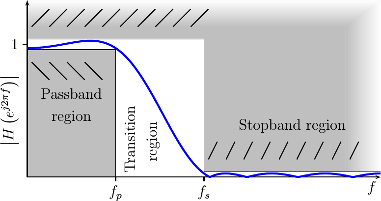
So, what is this symmetry, and how shall we exploit it? To understand that, let’s go back to the beginning and understand how digital filters, are designed.

To design a filter, the engineer must first determine a range of frequencies he wants the filter to “pass” (i.e. the passband), and another range of frequencies he wants the filter to “stop”. These two ranges tend to be disjoint, with a “transition band” between them. Within the stopband, the engineer must determine the “depth”, also known as how much attenuation the filter is to provide in this region. This can also be used as a criteria on how much (or little) distortion is allowed within the passband).

All of these criteria are easily illustrated in Fig 1 below.

Fig 1: FIR Filter Design Criteria

Given this criteria, the Parks and McClellan algorithm is well known for generating “optimal” filters. This filter design method produces filters that come closest to the filter design specification, as measured by the maximum deviation from the specification. There are two other realities with using this method. First, the filters designed by it all have an odd number of coefficients. Second, as designed they are all symmetric and non-causal.

These two characteristics follow the fact that the filter is specified with real, as opposed to complex or imaginary, criteria. That is, the desired filter’s frequency response is expressed as a real function of frequency.

Let’s think about this for a moment. We already know that if you have a sampled sequence, x[n], and apply a filter with impulse response h[k], then you will get the output y[n].

Fig 2: Convolution Operation

This operation is called a discrete convolution, and it defines the operation of any discrete-time filter. Fig 2 shows this operation pictorially, illustrating how the x[n] elements can be placed into a tapped delay line, multiplied by their respective h[k] coefficient, and then summed together to create the output y[n].

Further, if you apply this operation to a complex exponential, such as when

$x[n]=e^{j 2pi fn+jtheta}$

then the output of the filter is the same exponential, having only been multiplied by a complex value that is independent of time,

$y[n] = e^{jtheta}e^{j2pi fn} SUM h[k] e^{-j2pi fk}$

This complex multiplier is called the frequency response of the filter. It is defined by,

$H(e^{j2pi f}) = SUM h[k] e^{-j2pi fk}$

This is also the function we were specifying earlier in Fig 1 above. This should be familiar to you so far, as we have already discussed the importance of a filter’s frequency response.

Now consider what happens if we insist that this frequency response is a real function of frequency, just like we specified it above. We’ll use hs[k] and Hs to describe this constrained filter. If this filter has a real frequency response, then the frequency response function must be equal to its conjugate. We’ll start our proof there.

We can then replace Hs with its definition from above and shown in Fig 1, and then work the conjugate through the summation.

$SUM h[k] e^{-j2pi fk} = SUM h[k] e^{j2pi fk}$

Here, we note two things. First, hs[k] is real and so hs[k] is also equal to its own conjugate. Second, if we reverse the summation on the right via a variable substitution p=-k, then we have

$SUM h[k] e^{-j2pi fk} = SUM h[-p] e^{-j2pi fp}$

We’ll switch back to a summation over k for convenience of notation, although this “new” k value is just a dummy variable bearing no reference to the k three equations above. (Yes, I did get marked off for doing this by my instructor years ago.)

$SUM h[k] e^{-j2pi fk} = SUM h[-k] e^{-j2pi fk}$

Now reflect on the fact that this relationship must be true for all frequencies, f. That can only happen if

for all k. In other words, any filter with a real frequency response, such as those designed from a real frequency response criteria, will always be symmetric about the time axis, k.

Of course, this isn’t very useful to us, since any filter having non-zero values of h[k] for k<0 is non-causal and as such cannot be implemented: it depends upon the knowledge of future values of x[n]. The easy way to deal with this problem is to take the symmetric filter we just designed, and shift it so that it’s first non-zero coefficient is h[0].

Hence, we now have a filter with N non-zero coefficients, and where

This does nothing more than delay the operation of our filter in time–something the designer may not care about.

If you evaluate the frequency response of this adjusted filter, you’ll find its frequency response to be related to our earlier frequency response, by a linear phase term.

$H(e^{j2pi f}) = e^{-j pi fN }SUM h[k]e^{-j 2pi fk}$

The difference between the frequency response of the two filters, the one symmetric about zero and the offset but now causal filter, is a phase term that is linear in frequency. For this reason, filters of this type are often called linear phase filters.

But let’s go back a step, did you catch how this affects how we might implement this filter? If the filter remains symmetric such that,

then we can rewrite our convolution so it uses fewer multiplies.

y[n] = SUM h[k] ( x[n-k] + x[n+k-(N-1)] ) + h[M]x[n-M]

Fig 3: Convolution Operation Exploiting Coefficient Symmetry

This is a big deal! It’s a big deal because we now have half as many multiplies as we had before! We can even scale our filter such that the middle point of the filter, h[M], has some sort of “simple” value like (2^(K-1))-1 for a K bit word size, for one fewer multiply. Put together, we’ve just about doubled the capability of any filter we might wish to implement for only a minimal cost in additional logic.

You can see how this affects our operation in Fig 3. Notice how the tapped delay line containing the incoming signal is now folded in half. Further, before the multiply, there’s an addition where we add the pairs of signal data points together before multiplying by the common filter coefficient. You might also notice the single value on the right. This represents the coefficient in the middle–the one we’ll multiply by a constant value.

Now compare Fig 3 to Fig 2 and count the multiplies. See the difference? Instead of N multiplies, there are now (N-1)/2, or nearly half as many as we had before.

Now let’s take a look at how we might optimize our filter’s implementation to take advantage of this property.

C++ Implementation

Although this is an FPGA focused blog, sometimes it helps to consider an algorithm in a higher level language to understand it. So let’s spend a moment and review the C++ code describing our last implementation, and then show how this would change to exploit the symmetry inherent in most FIR filters.

As we presented it before, the slow filter C++ code worked by first adding a new data sample to a circular buffer.

double	FIR::apply(double dat) {
	int		i, ln;
	double	acc, *d, *t;

	m_data[m_loc++] = dat;
	if (m_loc >= m_len)
		m_loc = 0;

Then the filtering algorithm stepped through each filter coefficient, multiplying it by a corresponding data sample.

	acc = 0.0;
	d   = &m_data[m_loc];
	t   = &m_taps[m_len-1];
	ln  = m_len - m_loc;
	for(i=0; i<ln; i++)
		acc += *t-- * *d++;

Notice that the two indices go in opposite directions. This is an important feature of any filtering, implementation where the filter might not be symmetric. For symmetric filters, the direction the coefficients are read doesn’t really matter all that much.

The algorithm was made just a touch confusing by the fact that the data is kept in a circular buffer. As a result, the relevant data might cross the boundary of the circular buffer, from the right half to the left. If you split the loop into two parts, you can avoid checking for the buffer split within the loop itself.

	d   = m_data;
	ln  = m_loc;
	for(i=0; i<ln; i++)
		acc += *t-- * *d++;

Finally, the algorithm ended by returning the accumulated sum of products.

	return acc;
}

That’s the basic filtering algorithm that you can apply to implement any FIR filter. (Remember, for FIR filters longer than about 64-taps or so, FFT methods are faster/better/cheaper in software than the direct form presented above.)

Now, how would we modify this algorithm to create an implementation that would exploit the symmetry within our impulse response coefficients?

We’d start out exactly as before, by adding the new data sample to our input sample memory.

double	SYMFIR::apply(double dat) {
	int		i, ln;
	double	acc, *d, *t;

	m_data[m_loc++] = dat;
	if (m_loc >= m_len)
		m_loc = 0;

However, that’s about as far as we can go in common with the previous algorithm.

The next step is to calculate two pointers into the data–something we didn’t need to do before. The first, dpnew, will be a pointer to the most recent data that we just added into our buffer, while the second, dpold, will point to the oldest data in our buffer. Since the buffer has only as many samples within it as we have coefficients in our filter, we only need to check for wrap around once.

	dpnew = &m_data[m_loc-1];
	if (m_loc == 0)
		dpnew = &m_data[m_len-1];
	dpold = &m_data[m_loc];

We’ll also set a pointer to our coefficient memory.

	t = m_taps;

At each point through the summation, we’ll read two values from our data memory, one older *dpold and one newer *dpnew. We’ll then add these two values together, and multiply the result by the filter coefficient.

	do {
		double	presum = (*dpold++) + (*dpnew--);
		acc += *t++ * presum;

So far this is all very straight forward.

Where this C++ version gets difficult is when we try to handle pointer wrapping in our circular buffer. Unlike before, when we only had one pointer to check, we now have two pointers that might wrap as we work our way through memory. Rather than work through the math of separating this loop into three parts, I’ll just add a wrap check inside the loop.

		if (dpold > &m_data[m_len-1])
			dpold = &m_data[0];
		if (dpnew < &m_data[0])
			dpold = &m_data[m_len-1];
	} while(dpold != dpnew);

This loop will end before we get to the multiply in the middle of the filter. So, let’s handle it now and then return our result.

	acc += (*t) * (*dpold)
	return acc;
}

For those who might ask, yes, I do like redundant parentheses. That’s really beside the point, however.

The point here is that for an N point filter, where N is odd, we’ve just calculated the result using only 1+(N-1)/2 multiplies, instead of the N multiplies it would have cost us before.

This is the basic algorithm we’ll code up in Verilog in the next section. However, in Verilog we’ll use a memory in a circular addressing configuration. That way we don’t have to worry (much) about wrapping the pointers around. We will, however, need to worry about timing and pipeline scheduling.

Verilog Outline

When we first built our slow filter implementation, we used Fig 4 to illustrate how it worked.

Fig 4. A Time Multiplexed filter implementation

This diagram shows data coming in from the left, and going through two tapped delay lines. A selector then walks through each of the samples in the tapped delay line picking a data value. At the same time, a separate selector picks a value from the filter’s impulse response coefficients. These two values are shown multiplied together, accumulated, and then output.

To build this symmetric filter, we’re going to first break the tapped delay line structure into three parts, as shown in Fig 3.

Fig 5. Breaking the data tapped delay line into three pieces

The parts on the left and right will be implemented by block RAMs, and data will appear to “move” through the RAMs by just adjusting the indices used. The data point in the middle is point of symmetry for the filter. This point will not reside within either of the block RAMs. Instead, we’ll make this the last item read from the left block RAM, and place this item into the second block RAM on any new sample.

When a sample is provided, all the data will shift right by one. That will be our first step.

	always @(posedge i_clk)
	if (i_ce)
		dwidx <= dwidx + 1'b1;

Using this index we’ll write the new sample to the left data memory.

	always @(posedge i_clk)
	if (i_ce)
		dmem1[dwidx] <= i_sample;

We’ll read the mid-point sample from the last value read from this memory.

	always @(posedge i_clk)
	if (i_reset)
		mid_sample <= 0;
	else if (i_ce)
		mid_sample <= dleft;

Finally, we’ll write that mid-point sample to the right half of memory.

	always @(posedge i_clk)
	if (i_ce)
		dmem2[dwidx] <= mid_sample;

Notice that we are using the same write index for both halves of memory. We’ll have to deal with this a bit in our next step, since we are writing to the newest memory on the left, and half way through the memory on the right.

That will handle data movement, what about reading the data?

To read the data, we’ll set two data pointers–one to each block RAM–when any new sample comes in. These will initially point to the extreme locations in the memory, both the oldest and the most recent. These pointers will then walk, in unison, towards the center data point, as shown in Fig 5 above.

	always @(posedge i_clk)
	if (i_ce)
	begin
		lidx <= dwidx; // Newest value
		ridx <= dwidx-(HALFTAPS[LGNMEM-1:0])+1;
	end else if (not_done_yet)
	begin
		lidx <= lidx - 1'b1;
		ridx <= ridx + 1'b1;
	end

The next steps with the data are fairly straight forward. There’s not much magic in them. First we’ll read the data,

always @(posedge i_clk)
begin
	dleft  <= dmem1[lidx];	// Left memory
	dright <= dmem2[ridx];	// Right memory

then add the two values together,

	dsum <= dleft + dright;

then multiply them by the filter coefficient, filter coefficient,

	product <= dsum * tap;

and add the result to an accumulator.

	acc <= acc + product;
end

You may notice that we didn’t clear the accumulator, acc. We’ll have to come back to that. You may also notice we skipped some steps along the way, although this is the basic algorithm. So, let’s go back a bit.

We’re going to need to read the filter coefficient before we use it. This will involve resetting the index to the beginning of the coefficient memory,

always @(posedge i_clk)
if (i_ce)
begin
	tidx <= 0;	// Filter coefficient index

and then reading the next filter coefficient on every clock subsequent clock until we’re done.

end else begin
	tidx <= tidx + 1'b1;
	tap <= cmem[tidx];	// Filter coefficient index
end

At this point, our algorithm roughly looks like Fig 6 below.

Fig 6. The symmetric slow filter's block diagram

We read from each data block in opposite directions and added the two values together. We also read from our coefficient memory, and then multiplied the filter coefficient by the data sum. Finally, we accumulated the products together to create an output.

We’re still missing a couple items, though. For example, we need to multiply our mid-point by some value. Let’s fix that value to be 2^(M-1)-1, also known as the maximum positive integer that can be represented in M signed bits. This works because this sample value is usually (always?) the largest value in the filter.

always @(posedge i_clk)
if (i_reset)
	midprod <= 0;
else if (m_ce)
	midprod <= (mid_sample << (TW-1)) - mid_sample;

At least, that’s the basic idea of how we want the filter to work. Sadly, this simplistic approach to the algorithm is going to give us some headaches when we actually attempt to implement it in the next section. Why? Although we have a conceptual idea of what we wish to accomplish, the devil in this case lies in the details of how we handle the pipeline scheduling.

Verilog Implementation

When I first set out to implement this filter, I thought I might just quickly modify the generic slow filter I had presented earlier. This is basically what I just presented above in the last section. I’m mean, all that’s required is two memory reads, a sum and then the filter is identical to what it was before. It’s that simple, right?

No. It isn’t.

As a measure of difficulty, consider this: I’ve gotten to the point where implementing a basic DSP component like this has become fairly easy and routine. I therefore gave myself two days to do the task, and even then I didn’t work on it full time for both days. Much to my surprise, I almost didn’t finish the task within the two days I’d given to myself.

Why not?

It wasn’t that the filter was really all that hard to implement, but rather the problem was scheduling the pipeline. To understand this, let’s work from the fixed points in the schedule.

The first fixed points are the memory reads. In order to make certain the design tools place the data and filter coefficients into block RAM, they can only be accessed in the simplest of ways. Specifically, each RAM must takes one clock cycle to read where you do nothing else with the value read. Yet moving the time the data were valid from the clock in the slow filter, to the next (i.e. following the summation) made for all kinds of havoc within my design.

In a humble admission, I’ll admit that I almost pulled out the formal methods to formally verify the design after I struggled so hard getting this to work within the test bench. It seems I’ve gotten hooked on how easy it is to get a design to work using formal methods. (Yes, it is possible to formally verify a digital filter using formal methods. The problem is that the multiply makes the application of formal methods difficult. I’ll leave this concept for another day, though, specifically for some time after I discuss the concept of abstraction in formal verification.)

In the end, in order to get the following design to work I had to work through the design and its test bench one clock at a time, verifying every value along the way until all of a sudden the design passed. While I was successful, I do have to admit that my success took more work than I expected. Shall we just say my performance at the task just wasn’t as graceful as I might have liked?

The key to the success of this design lies in the pipeline schedule. So, as I was building this algorithm, I scribbled out the pipeline schedule diagram shown in Fig 7.

Fig 7. Initial Pipeline Schedule

If you remember from our prior discussions of these charts, values are shown in the column in which they are valid. Hence i_ce is true on the first clock of our cycle. At that same time, the sample value, i_sample, the data write index (dwidx), mid-point sample from the last time through (mid_sample), and the final data value from the left block RAM (dleft) are also valid. On the next clock to the right, the data values may now be read from memory, hence dmem1[dwidx] is valid and so forth. On this clock also I’ll raise an m_ce signaling flag so I know where I am in this portion of the pipeline.

I’ve taken the time to show particular anchor points to this diagram in red. These are the points we worked out above in the last section. They are immovable in the pipeline. Hence, following the m_ce (first memory read valid) cycle there’s a first data valid cycle where d_ce is high. This will be the first of many such cycles. This is followed by a summation cycle, s_ce, when the first data sum is true. This is then followed by a product cycle, p_ce, when the first data product is true and so on.

The items in black are the ones I really struggled to get right. In particular, the first filter coefficient value doesn’t have to be valid until s_ce clock. That means its index must be valid the clock prior and not the clock prior to that. This one little difference marked the root of my problems.

But let’s get to these difficulties in order.

The first order of business is to allow the user to update the filter’s coefficients. This is almost the same exact code as we discussed earlier, so it really doesn’t need much comment.

	generate if (FIXED_TAPS)
	begin : SET_FIXED_TAPS

		initial $readmemh(INITIAL_COEFFS, tapmem);

	end else begin : DYNAMIC_TAP_ADJUSTMENT
		// Coef memory write index
		reg	[(LGNMEM-1):0]	tapwidx;

		initial	tapwidx = 0;
		always @(posedge i_clk)
			if(i_reset)
				tapwidx <= 0;
			else if (i_tap_wr)
				tapwidx <= tapwidx + 1'b1;

		if (INITIAL_COEFFS != 0)
			initial $readmemh(INITIAL_COEFFS, tapmem);
		always @(posedge i_clk)
			if (i_tap_wr)
				tapmem[tapwidx] <= i_tap;
	end endgenerate

The next order of business is to move our data pipeline. This happens any time a new sample is sent to the filter, as indicated by i_ce being high.

As you may recall, the global pipeline strategy works quite well for digital filter. Within this design, however, we’ll be using a traveling CE approach as you saw in Fig 7 above.

As part of this new sample routine, we’ll increment a data write index on every new sample.

	initial	dwidx = 0;
	always @(posedge i_clk)
	if (i_ce)
		dwidx <= dwidx + 1'b1;

There is no reset on this index, despite the initial value. This lack of a reset allows the filter to be cleared and flushed by holding the i_reset and i_ce lines high, while also forcing i_sample to be zero for as many clock cycles as the filter has taps.

We’ll also write our new sample to the first memory bank,

	always @(posedge i_clk)
	if (i_ce)
		dmem1[dwidx] <= i_sample;

our midpoint sample to the second memory bank,

	always @(posedge i_clk)
	if (i_ce)
		dmem2[dwidx] <= mid_sample;

and we’ll set our midpoint sample to be the last sample read from the first memory bank, or dleft as I’m going to call it with reference to either of Figs 5 or 6 above.

	always @(posedge i_clk)
	if (i_reset)
		mid_sample <= 0;
	else if (i_ce)
		mid_sample <= dleft;

Since mid_sample doesn’t need to be constrained to ultra-simple memory logic, it can be sensitive to the reset. This will halve the number of clock cycles it will take to clear this filter during a reset, since these zeros will then feed the second half of memory.

The next signal, pre_acc_ce, is the one we are going to use to control whether or not to accumulate a new product into our accumulator. This is the control value that will also keep us from accumulating past the last valid coefficient in our filter. For this reason, we start out by counting how many coefficients are remaining.

	assign	taps_left = (NTAPS[LGNTAPS-1:1]-tidx);
	assign	last_tap_index = (taps_left <= 1);

We’ll also calculate a flag to tell us whether or not we are at the last data index.

	assign	last_data_index= (NTAPS[LGNTAPS-1:1]-tidx <= 2);

Both of these values are referenced to the pipeline cycle where the index is valid. What that means, though, is that this measurement needs to be propagated to through the pipeline. This is the purpose of pre_acc_ce, the “pre” calculation of whether the accumulator should be updated. On any new data, pre_acc_ce[0] gets set to 1'b1. This starts the beginning of the accumulator pipeline.

	initial	pre_acc_ce = 4'h0;
	always @(posedge i_clk)
	if (i_reset)
		pre_acc_ce[0] <= 1'b0;
	else if (i_ce)
		pre_acc_ce[0] <= 1'b1;

It then stays at one until the index for the last coefficient.

	else if ((pre_acc_ce[0])&&(!last_tap_index))
		pre_acc_ce[0] <= 1'b1;

Here we get to one of the surprises of the algorithm. Because the coefficient index and the data index are off by one cycle, this last_tap_index value isn’t a sufficient indicator of when to turn the pre_acc_ce value off. Instead, we’ll turn it off as long as we aren’t starting around again on the next incoming sample.

	else if (!m_ce)
		pre_acc_ce[0] <= 1'b0;

This pre_acc_ce value now needs to be propagated through our pipeline. We’ll use a simple shift register structure for this purpose.

	always @(posedge i_clk)
	if (i_reset)
		pre_acc_ce[3:1] <= 3'b0;
	else
		pre_acc_ce[3:1] <= { pre_acc_ce[2:1],
			((m_ce)||((pre_acc_ce[0])&&(!last_tap_index))) };
	// Where ...
	// pre_acc_ce[0] means the data index is valid
	// pre_acc_ce[1] means the data values are valid, tap index is valid
	// pre_acc_ce[2] means the data sum and tap value are valid
	// pre_acc_ce[3] means that the product is valid

We can now interpret pre_acc_ce as follows. If pre_acc_ce[0] is true, the data index is valid. If pre_acc_ce[1] is true, the data values are valid. If pre_acc_ce[2] is true, the sum is valid and if pre_acc_ce[3] is true then the product is valid and may be accumulated.

You’ll see how this works more in a moment.

We’ll next focus on the data read indices. These will continue to follow the left and right convention from Figs 5 and 6 above. Hence we’ll have a left index, lidx, and a right index ridx. On any reset, these are set to zero, although this is really more for form than anything else.

	initial	lidx = 0;
	initial	ridx = 0;
	always @(posedge i_clk)
	if (i_reset)
	begin
		lidx <= 0;
		ridx <= 0;

Then, on any new sample, the left data index, lidx is set to point to the newest value just written to memory. The right half data index is a touch more complicated–and took me many trials to get right. This index is given by back tracking from the oldest value by half our filter length. This would’ve been the entire size of the second memory, save that we are forcing the memory to have a power of two size, while the NTAPS can be any arbitrary odd number.

	end else if (i_ce)
	begin
		lidx <= dwidx; // Newest value
		ridx <= dwidx-(HALFTAPS[LGNMEM-1:0])+1;

As a last step, we’ll step the indices as long as this isn’t the last data index. The left index steps backwards from the newest value to older values, while the right index steps forwards from the oldest index to the newer index.

	end else if ((m_ce)||(!last_data_index))
	begin
		lidx <= lidx - 1'b1;
		ridx <= ridx + 1'b1;
	end

Keep in mind, the last_data_index criteria here is key. In particular, we are about to read the left data value, dleft, from the left memory based upon this index. This will turn into the mid point value on the next sample. For this reason, the indices cannot be allowed to just free run.

The second remarkable piece of this logic is the m_ce criteria. Our last_data_index flag depends upon the cofficient index, not the data index. This coefficient index isn’t (yet) valid on the m_ce cycle. Hence, we need to continue to walk the index forward even before the first tap index is valid. (Yes, this was another one of those details that surprised me as I built this.)

A very similar piece of logic is used to determine the filter coefficient index.

	initial	tidx = 0;
	always @(posedge i_clk)
	if (i_reset)
		tidx <= 0;
	else if (m_ce)
		tidx <= 0;
	else if (!last_tap_index)
		tidx <= tidx + 1'b1;

While it might look like we might just let this value run as well, keep in mind that we are using the filter coefficient index as an indicator of when to stop accumulating. For this reason, this index also stops at the end of the coefficient memory.

That’s the data and coefficient index calculation. Let’s move on to the memory read cycle(s). We’ll mark this cycle with an m_ce flag, as shown in our pipeline schedule in Fig 7 above, indicating that this is the first cycle the memory data is valid.

	initial	m_ce = 1'b0;
	always @(posedge i_clk)
		m_ce <= (i_ce)&&(!i_reset);

On this cycle we’ll read from the two block RAMs of data.

	initial	dleft  = 0;
	initial	dright = 0;
	always @(posedge i_clk)
	begin
		dleft  <= dmem1[lidx];
		dright <= dmem2[ridx];
	end

Following the outline in Fig 7, the next pipeline cycle and flag is the data valid cycle, d_ce. This follows the m_ce flag, and like it this is only valid for one clock cycle.

	initial	d_ce = 0;
	always @(posedge i_clk)
		d_ce <= (m_ce)&&(!i_reset);

Now we can read the coefficient index,

	initial	tap = 0;
	always @(posedge i_clk)
		tap <= tapmem[tidx[(LGNTAPS-2):0]];

and add the data values together.

	initial	dsum = 0;
	always @(posedge i_clk)
	if (i_reset)
		dsum <= 0;
	else
		dsum   <= dleft + dright;

We’ll use the s_ce signal to mark that the first data summation is valid.

	initial	s_ce = 0;
	always @(posedge i_clk)
		s_ce <= (d_ce)&&(!i_reset);

The data sum times the filter coefficient is our product value. If this looks familiar, it should–this matches the slow filter code, and was drawn from it. This should also matches our discusion in the last section.

	initial	product = 0;
	always @(posedge i_clk)
		product <= tap * dsum;

The midprod value is different. midprod is the product of the mid-point sample, mid_sample times the maximum positive integer value that fits in TW bits, or 2^(TW-1)-1.

	initial	midprod = 0;
	always @(posedge i_clk)
	if (i_reset)
		midprod <= 0;
	else if (m_ce)
		midprod <= { {(OW-IW-TW+1){mid_sample[IW-1]}},
					mid_sample, {(TW-1){1'b0}}}
				-{ {(OW-IW){mid_sample[IW-1]} }, mid_sample};

That then leads us right into the accumulator. There are three parts to this. First, we’ll set it to zero on any reset.

	initial	r_acc = 0;
	always @(posedge i_clk)
	if (i_reset)
		r_acc <= 0;

Second, on the s_ce cycle (see Fig 7 above), we’ll initialize this accumulator to be our midpoint product.

	else if (s_ce)
		r_acc <= midprod;

Third, on every subsequent sample with a valid product, we’ll add the product to our accumulator.

	else if (pre_acc_ce[3])
		r_acc <= r_acc + { {(OW-(IW+TW)){product[(IW+TW-1)]}},
						product };

Finally, on the same sample that we initialize our accumulator with the mid-point product, we’ll set our result to be the last value that had been in the accumulator.

	initial	o_result = 0;
	always @(posedge i_clk)
	if (s_ce)
		o_result <= r_acc;

In a similar fashion, we’ll set our output clock enable strobe, so that the rest of the signal processing pipeline can continue to follow the global CE strategy.

	initial	o_ce = 1'b0;
	always @(posedge i_clk)
		o_ce <= (s_ce)&&(!i_reset);

endmodule

That’s all it takes to build a symmetric filter running N times slower than the system clock.

Perhaps the biggest lesson learned to draw from this discussion is how dependent I was on the simulator to get particular values right. For example, did you notice the strange logic on pre_acc_ce? Or how about the fact that the last_data_index compared against two instead of zero or one? Or perhaps that the taps_left calculation didn’t depend upon the total number of taps, but rather (N-1)/2? (Remember, N, the number of coefficients, must be an odd number.) All of these values were determined with the help of running many simulations.

Test Bench Performance

When it comes to building the test bench for this system, there wasn’t a lot of work to be done–thanks to the work we did building a generic filtering test bench some time earlier. Even better, if you meld this test bench driver against the test bench driver for the slow filter,

meld slowfil_tb.cpp slowsymf_tb.cpp

you’ll see only a very small, limited number of (key) differences. While most of these are concerned with adjusting filter length related parameters, there is one particular difference worth commenting on. That difference is in the testload() function.

As you may recall from our discussion of the generic filtering test harness, the testload method allows us to load coefficients into the filter, and then test the impulse response of the filter to insure those coefficients were loaded correctly. In our case, this also gives us a chance to verify that the filter’s response is symmetric as we had intended.

        void    testload(int nlen, long *data) {
		// Load the given coefficients into the filter
		load(nlen, data);

		// Loop through and test each coefficient
		for(int k=0; k<2*NTAPS(); k++) {
			int	m = (*this)[k];

If the coefficient comes before the midpoint, it should match the data given to this function and passed to load above.

			if ((unsigned)k < MIDP)
				assert(data[k] == m);

Likewise if this is the midpoint, then the coefficient should be equal to the fixed value, (1<<(TW-1))-1, where TW remains the maximum number of bits in any coefficient.

			else if (k == MIDP)
				assert(m == (1<<(TW()-1))-1);

On the other side of the midpoint, the coefficients should read back in reverse order. In other words, here is where we check the symmetry.

			else if (k < NTAPS())
				assert(m == data[NTAPS()-1-k]);

Finally, anything beyond the number of taps in the filter should return zero.

			else
				assert(m == 0);
		}
        }

Once this is accomplished, we can now use our test bench structure to measure the filter’s performance against the lowpass filter configuration we’ve been testing against. The result is a stopband rejection roughly between -55 and -54 dB, which is just what we were expecting.

That’s not that bad, especially if you consider that we only used half as many clock cycles as the last slow filter we studied.

Conclusion

This filter implementation marks one of those times where a little bit of engineering up front will spare you a lot of design resources later. That’s why we added a touch more mathematics above to what we had done before. Sure, our implementation is a touch more complicated than the last slow filter. But look at what we gained: twice the performance! That’s what makes this filtering implementation valuable. How applicable is it? This approach applies to all filters designed via the optimal Parks and McClellan filter design algorithm. In other words, this is almost a universally applicable optimization among FIR filter implementations.

As I mentioned above, we have yet to discuss many other types of filtering implementations. Perhaps this simplest filter to build next would be a half band filter. For certain filters, a half band filter implementation can be built for half again as many resources as we just used.

We’ll have to come back again on another day, though, in order to demonstrate and discuss some of these other filters.