I’d like to spend some time discussing Digital Filtering on this blog.

This is going to be a bit of a difficult topic, however, in that I don’t intend to discuss how to design a Digital Filter, nor do I intend to discuss how to evaluate the design of a digital filter, nor do I intend to discuss aliasing. These are all vital topics necessary for understanding what a digital filter is, as well as understanding whether or not a digital filter even works. They are also vital topics to understand when comparing the performance of one digital filter with that of another. However, these are really topics for a different course.

For now, it’s worth understanding that a digital filter implements a discrete convolution, and that such discrete convolutions are provably the only signal processing operations that are both linear and shift invariant. This makes them a very important part of any discussion of digital signal processing (DSP).

It’s also worth noting that any student of digital signal processing should be able to recognize when a digital filter is causal, stable, when it has linear phase, and when it has a finite (FIR) or an infinite (IIR) impulse response.

Our focus in this blog is going to be on how to debug a digital filter so that you can know it works. To get there, though, we are going to have to describe some filters so that we have something to debug. Filters we discuss, together with any test or debugging logic, will be placed on GitHub here.

For today, let’s just look at two very simple filters: the simplest non-trivial FIR filter that I know of, and a simple recursive averager (a type of IIR filter) that I have found to be very useful.

Simple FIR Filter

The first filter we are going to look at may well be the simplest FIR filter you will ever come across. It simply averages adjacent samples together.

The code to implement this equation is likewise just as simple:

initial	delayed = 0;
always @(posedge i_clk)
	if (i_ce)
		delayed <= i_val;
always @(posedge i_clk)
	if (i_ce)
		o_val <= i_val + delayed;

This filter is useful for many reasons. For example, unlike many other filters that you may study, this filter requires no multiply (DSP) resources within the FPGA. The output only grows by one bit. Further, this filter can also handle incoming samples at up to the full system clock rate for the FPGA. Those are the good qualities of this filter.

It is also, however, a very difficult filter to use successfully simply because its frequency response rarely describes the performance that you want. It doesn’t have a sharp cut off. Its taps and length are fixed. Indeed, you might find this filter that we’ve just implemented to be quite useless.

Before you give up on this simplest filter, consider what would happen if you cascaded several of these filters together–one right after the other. For example, suppose you ran your signal through ten of these filters in succession. You would get a filter with a much deeper stopband.

This is the comparison shown in Fig 1 below. In it, you can see the predicted frequency response of our original simple filter above, as well as a similar predicted frequency response for the filter that would result from applying that same filter ten times in a row. Both filters have been normalized so as to have a unity response to anything at zero frequency.

Fig 1:

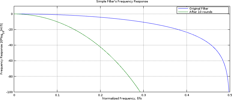We’ll need come back to this later, when it’s time to determine whether either filter actually achieves this predicted frequency response.

While this new cascaded filter is starting to have a nicely acceptable stop band, nothing remains that might be considered a flat “pass” band anymore. Still, the cascaded filter is easy enough to build and costs so few resources that whenever a cascaded filter of this type can be used, even if as only a component of other filters, it is often very valuable to do so. Therefore, this simple filter finds its best and greatest application in being a component of other, more powerful, filters.

Simple IIR Filter

The next super-simple filter that I’m going to present is an IIR filter. Specifically, let’s look at a recursive averager. A recursive averager keeps an average value at all times, and only adjusts that value with any input. Specifically, I like to think of it as a weighted sum of some percentage of the new input sample plus the remaining percentage of the last average.

Perhaps an equation will help. In symbology, a recursive averager is just:

Where we keep to the standard conventions of n being the sample number, x[n] being our input and y[n] being our output. The new variable here, alpha, is our means of adjusting how deep or sharp this filter is. This is a value between zero and one. If alpha is one, no averaging takes place. The closer alpha is to zero, however, the more the filter will average the input and the longer it will take to converge to an average. Likewise, the closer alpha is to zero the less noise the filter will admit to the average estimate.

With a little manipulation, we can rearrange this filter into something that’s really easy to compute.

Then, if we insist that alpha be a negative power of two, we can replace the multiply above with a right shift:

You’ll want to use an arithmetic shift here, to mak certain the sign propagates in the case where the difference is negative.

This leads us to our first design choice: How many clocks can we use to calculate an answer? In particular, this recursive averager is going to require a subtraction followed by an addition. Both of these operations need to complete before the next sample. You can either try to place this all within a single system tick, or split it between two separate ticks.

If you have new data samples present on every clock tick, you will need to try the combinational approach I’m going to present below, stuffing all of the logic into a single clock tick. This has the unfortunate consequence of limiting your system clock speed.

On the other hand, if your data samples will always have at least one unused clock between them, then you could take one clock tick to calculate the difference, x[n]-y[n-1], and another to update the running average, y[n].

If we suppose that we must do this all within a single clock tick, the following code will implement this recursive averager. In the code below, AW is the number of bits in the averager, and IW is the bit-width of the input.

wire	signed	[(AW-1):0]	difference, adjustment;

// The difference is given by x[n] - y[n-1]
assign	difference = { i_data, {(AW-IW){1'b0}} } - r_average;

// The adjustment is the difference times alpha
assign	adjustment = { {(LGALPHA){(difference[(AW-1)])}},
			difference[(AW-1):(AW-LGALPHA)] };
always @(posedge i_clk)
	r_average <= r_average + adjustment;

assign	o_data = r_average;

You may notice that I could have used the Verilog shift operator and did not. Had I done so, then the adjustment value could have been set with:

assign	adjustment = difference >>> LGALPHA;

So, how did we do? We’ll need to come back and test this later to know for certain. That in itself is going to need to take some thought. Just what is the best way to test a filter? For now, you can see in Fig 2. how good we should be doing—if we had truly infinite precision arithmetic.

Fig 2:

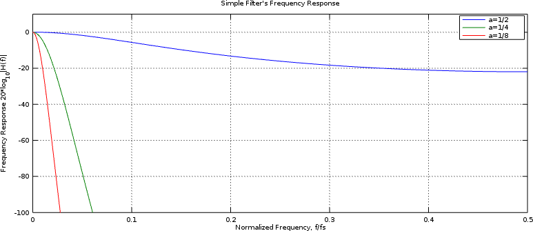Later, it would be nice to come back and generate this frequency response curve as a result of measuring how well the filter actually does. Parameters that will impact this measurement include not only how many bits are allocated to the input and output (averager) values, but also how big the input value truly is.

Unlike the simple FIR filter above, applications for this simple IIR recursive averaging filter abound just about everywhere.

Want to measure a histogram? Set this up to be an unsigned recursive averager and then place a 1 into this filter every time your data is within the bin of interest.

Want to drive an automatic gain control circuit? Compare the absolute value of your signal against a fixed threshold. Set the averager for unsigned values, and then if your signal’s amplitude is too high you can average a 1 into this averager. If the result is too low, average a 0 into this averager. You can then use the result to know if you should turn the gain in your circuitry up or down.

You could also use this to remove any fixed gain in your circuitry.

Indeed, you could even use this circuit coupled with a CORDIC to measure a single bin (or more) of the frequency response of your system.

This filter is exceptionally versatile as a cheap low-pass filter. As an example of that versatility, it also finds applications in phase lock loops!

These are all other topics, though, that we’ll need to come back to another time.

Conclusion

Yes, those are the two simplest (non-trivial) filters I know.

Sadly, though, we’re not yet in a position to test these filters to know that they work. As a result, we’ll need to come back to the topic of digital filtering once we discuss how to properly test a digital filter. Some of those techniques will depend upon being able to use a CORDIC–something we have yet to present on this blog. We’re also going to need to have a thorough understanding of quantization noise, another thing we’ll have to come back and discuss.

This is by no means our final digital filtering, discussion either! Many, many other FPGA filtering topics remain. These include:

• How to estimate a filter’s logic resource usage

• How to build the cadillac of all filters: a dynamic filter whose filter taps can be set at run time.

• And then how to build more realistic filters that will actually fit within your FPGA’s logic resources.

Do you get the feeling that digital filtering is a complex topic? Since it is the most basic DSP operation, we’ll need to spend some time going through it. Perhaps some well written examples will help to make this complex topic make more sense.