Measuring the frequency response of a filter under test

We’ve slowly been building several digital filtering Verilog implementations on this blog. For example, we’ve presented a generic Finite Impulse Response (FIR) filter implementation, and even a cheaper version of the same. I’d like to move forward and present some other filter implementations as well, but I haven’t finished presenting the test bench for the filters I have presented. Therefore, we’ve also been slowly building up to a test bench by building a test harness that we can use to prove that not only these two filter designs work as designed, but also that other filter designs we might build later work as designed.

In our last post discussing digital filtering, we presented a generic test harness that can be used when building test benches for various digital logic filters. This test harness verified a number of things regarding a filter, to include measuring the filter’s impulse response as well as making sure that the filter’s internal implementation didn’t overflow.

For the verification engineer, this isn’t enough.

Why not?

Fig 1. Lowpass FIR requirements

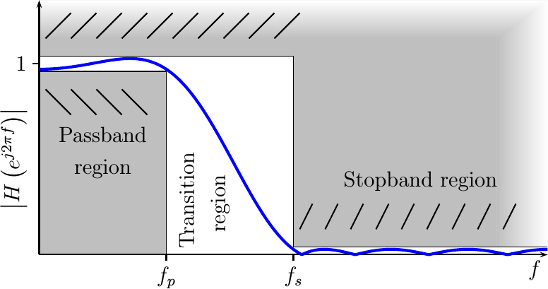Well simply because the requirements for a filter, such as might be shown in Fig 1, are specified in terms of the filter’s frequency response–not its impulse response. If you want to answer the question of whether or not a particular implementation meets your criteria, then you need to measure the frequency response of the filter you are creating. Otherwise how will you be certain that your filter works as advertised? That it accomplishes the function it was designed to perform?

Today, therefore, let’s spend some time discussing what the frequency response of a filter is, why it is important, and then examine how one might go about measuring it.

The Frequency Response Function

There’s really some wonderful math underpinning FIR filters in general. Perhaps you remember some of this from our earlier “What is a Filter” discussion. Today, we’ll just outline that math, and then show how it naturally leads to this concept of a frequency response.

The roots of an FIR filter lie within the concept of a linear operation on a data stream. If that linear operation, whatever it is, also happens to be shift invariant then the operation can be described by a convolution between the input, x[n] and the filter’s impulse response function, h[n].

When dealing with the filters that digital logic can create, reality lays two additional constraints onto these filters. First, h[k] for k<0 must be zero. This is another way of saying that the filters is causal–it doesn’t know anything about inputs that haven’t yet been received. The second criteria is that h[k] must be an integer (i.e. quantized).

We’re also going to assume a third criteria for today’s discussion, which is that h[k] must be zero for k>= N samples. This is another way of saying that h[k] must only be non-zero for a finite number of samples, from k=0 to k=N-1. For this reason, this type of filter is called a Finite Impulse Response (FIR) filter.

All of this is just a quick background refresher regarding the properties of the types of filters we are looking at. These properties lead into the development of the filter’s frequency response function.

The idea of the frequency response of a filter is fairly simple: what response does the filter return when a complex exponential is fed to the filter as its input.

By complex exponential, I mean more than the Euler’s formula Wikipedia discusses under that term. Instead, I am referring to a function such as

This function has a unit magnitude and it steps forward by a constant phase shift between samples. It expands, via Euler’s formula, into sine and cosine components–we’ll use this property later on.

So let’s find out what happens to an input of this type when our filter is applied to it.

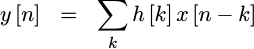
We’ll start with the equation for a linear, shift-invariant system: a convolution.

We’ll then replace x[n] with a complex exponential function, exp(-j 2pi fn), for some frequency -1/2 < f < 1/2,

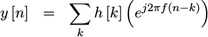and then we’ll simplify and rearrange terms,

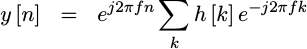Did you notice how, after we rearranged the terms, the summation no longer depends upon time, n, anymore? Instead, the internal part of the summation depends only upon k–the index variable for the summation. In other words, the value within the summation depends upon the frequency, f, and the filter’s coefficients (it’s impulse response, h[k]) alone, and once summed the value is a constant for all time, n. We’ll use H(e^{j2pi f}) to represent this constant,

This H(e^{j2pi f}) function is called the frequency response function of our filter, h[k].

This frequency response function allows us to represent the output of our filter, whenever the input is a complex exponential, by that same input complex exponential times the frequency response function, or

But, why is this so important?

It’s important simply because we now have a way of describing how our filter interacts with its inputs in a fashion that is independent of the input. Further, the operation is a straight multiply–much simpler than the convolution we started with. Hence, any input that can be described as a sum of complex exponentials (that’s all of them), will have an output which is also described by a sum of complex exponentials–only those exponentials will now have a weighting given by H(e^{j2pi f}).

Indeed, this representation is so important that filters are most often specified by the frequency response they are required to achieve. Determining the frequency response our filter actually implements, and hence whether or not it has achieved its design requirements, is the purpose of the frequency response measurement function of our generic filter test harness–the topic for today’s discussion.

How shall we calculate it?

The common means of calculating the frequency response of a filter is to take a Fourier transform of its impulse response. This follows directly from the discussion above developing what a frequency response is in the first place. The Fast Fourier Transform (FFT) is a computationally efficient means of evaluating a frequency response from an impulse response. Chances are you will need to do this as part of your filter design process.

When you do so, you’ll want to make certain that your FFT size is about 8-16x greater than the number of taps (coefficients) in your filter. More than 16x usually doesn’t buy you anything, and anything less than 4x hides details. No window function is required, and indeed no window function should be used in this process. The filter coefficients themselves should have any necessary window built into them.

This common method works great until you want to know whether or not your filter as implemented achieves the frequency response you are expecting. To actually measure the frequency response a filter produces requires actually placing a complex exponential input into the filter, and then plotting the output that you receive as a result. The details of how to do this using Verilator will be discussed in our next section.

Filter Harness Code for measuring the Frequency Response of a Filter

At this point, we’ve now explained both what a filter’s frequency response function is, as well as how it is commonly calculated (not measured). Let’s now look into how we might actually measure this frequency response given a particular filter’s implementation that may, or may not, be working.

Since the filter implementations we are working with are all real implementations, then we’ll have to do a touch of pre-work in order to estimate their frequency response to a complex exponential input.

The first part of this pre-work will be to deal with the phase of our measurement. You may recall from above that if

then

For our testing below, we’ll define x[0] to be the first sample in any individual test. Yes, I know, this redefines time zero from one test input to the next, but it does make a good reference for developing the inputs. What this means, though, is that y[n] isn’t defined entirely by our new values until y[N-1] since anything earlier would reference an x[n] with n<0 that might have been part of our last test vector. Worse, the filter response at y[N-1] has a phase term within it in addition to the frequency response term we want.

This initial phase term needs to be removed if we want to measure H(e^j2pi f).

So let’s suppose we instead provided an input of

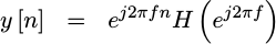
Our output at y[N-1] would then be

If we define phi to be

then

as desired.

The next problem to deal with is the fact that our filter is only real valued: both the inputs, the coefficients, and the multiplies only work on real numbers. How then shall we get the results from a complex operation? In this case, we need to break H(e^{j2pi f}) into it’s real and imaginary components using Euler’s formula:

These two terms contain only real numbers and real operators, even though the measured result will be complex. The first term has a cosine wave as an input, the second a sine wave. The second term needs to be multiplied by j, the square root of negative one, upon completion. However, by splitting this filter into two parts, one for the real part of the input and one for the imaginary part of the input, we can now generate this complex value with two test vectors–both of which are real and so both of which our implementation can process.

Hence, for every frequency we are interested in (except zero), we’ll apply two test vectors to our input and examine the resulting output.

Now that we have a vision for how to proceed, it’s now time to build our frequency response estimation function. This will be part of the Verilator based test harness we discussed earlier. As such, it is a C++ function (not a Verilog module), but yet we will use it to evaluate our various Verilog filter implementations.

Further, we’ll build this response estimator using the filter test harness apply() function–a function that returns the response of the filter to a given test input. As we discussed last time, this function differs from the similar test() function in some critical ways. First, the test() function resets the filter to a known initial state, whereas apply() just uses the filter in the state it was last left in. Second, the test() function quietly adds input samples to compensate for any delay internal to the filter, whereas the apply() function does not. As a result, we’ll need to add these extra samples ourselves below. Still, using the apply() function will give us some confidence that the filter will properly and naturally flush its state from one input to the next–something the rest of the test harness has yet to verify.

The parameters to this function are much as you might expect. There’s the number of frequencies, nfreq, that you’d like to use to cover the frequency band from 0 to the Nyquist frequency, 1/2. As I mentiond above, this number should be between 8x and 16x the filter’s length. There’s also a complex array pointer, rvec, to hold the frequency response once it’s been estimated. Those are both straightforward. Likewise the optional filename, fname, to save any results into is also straightforward. Perhaps the only remarkable item is the magnitude of the sine wave, captured in mag. A mag of 1.0 will cause us to create a sine wave having the maximum integer magnitude the number of input bits, IW, will allow. Anything less than one will scale the sine and cosine waves proportionally.

template<class VFLTR> void	FILTERTB<VFLTR>::response(int nfreq,
		COMPLEX *rvec, double mag, const char *fname) {

We’ll need to declare some variables to make this happen. The first, nlen is the number of coefficients in our filter. The next, dlen, is the same but captures the number of data samples we’ll need to send to apply() and so it requires the number of delay cycles between any input sample and the first associated output from the filter. We’ll use the data pointer to point to an array into which we can store both our outgoing data (test vectors to be sent to the filter), and incoming data (the response from the filter to the test vector). Finally, df will hold the value of our frequency step size.

	int	nlen = NTAPS(), dlen = NTAPS()+NDELAY();
	long	*data = new long[dlen];
	double	df = 1./nfreq / 2.;

As we discussed above, mag is the requested magnitude of the sine wave test vector, running from 0.0 to 1.0. We’ll use that number here to scale the actual magnitude we’ll use for our complex exponential input vectors.

	mag = mag * ((1<<(IW()-1))-1);

At this point, we can start walking through frequencies and making measurements. As I mentioned above, this isn’t the most efficient means of calculating a filter’s frequency response, but this will be a means of measuring it.

dtheta is the phase difference from one complex exponential sample to the next.

	for(int i=0; i<nfreq; i++) {
		double	dtheta = 2.0 * M_PI * i * df,
			theta=0.;

We’ll begin our complex exponential sample sequence at the phase we calculated above.

		theta = -(NTAPS()-1) * dtheta;

Then we’ll walk through the input vector and set it based upon a cosine function. This test vector should give us one real component of the filter’s frequency response.

		for(int j=0; j<dlen; j++) {
			double	dv = mag * cos(theta);

			theta += dtheta;
			data[j] = dv;
		}

Once we apply() the filter to this test vector, we’ll know the real component of the frequency response at this particular frequency. Note how we remove the magnitude scale factor below as well.

		apply(dlen, data);
		real(rvec[i])  = data[dlen-1] / mag;

We can then repeat this same process for the sine wave input in order to get the imaginary component of our measured frequency response. We’ll do this for all but the zero frequency, which is already known to be zero for any filter with real coefficients.

		if (i > 0) {
			if (debug) { /* ... */ }

			theta = -(NTAPS()-1) * dtheta;
			for(int j=0; j<dlen; j++) {
				double	dv = mag * sin(theta);

				theta += dtheta;
				data[j] = dv;
			}

			apply(dlen, data);
			imag(rvec[i])  = data[dlen-1] / mag;
		} else
			imag(rvec[i] = 0;

Once we finish our loop across frequencies, all that’s left is to close up, free any data we’ve allocated, and we’re done. This includes writing the measured frequency response out to a file–but that section is simple enough that we can skip any discussion of that part. See the code for the overall test harness, or the discussion of how to debug a DSP algorithm should you have any questions about this step.

		if (debug) { /* ... */ }
	}

	delete[] data;
	// ...
}

How well does this approach work?

Fig 2 below compares three filter frequency response functions against each other.

Fig 2. An example estimated frequency response

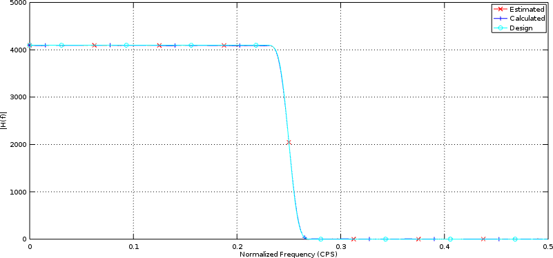All three are measures of the same filter coefficients, only measured in different fashions. The first, the estimated response, is the frequency response derived from the frequency response estimation code we just presented above. The second is the result of an FFT applied to the filter’s coefficients. The third line above shows the filter, as designed, but before we truncated any of the coefficients to twelve bits.

Perhaps a more revealing chart, however, would be Fig 3 below, which compares the same functions in Decibels.

Fig 3. Examining a filter's frequency response in Decibel's

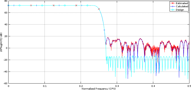In this example, you can see the effect that truncating the filter’s coefficients had on our initial design.

In both examples, however, the calculated and the estimated charts lie on top of each other–giving us reason to believe that our method above is trustworthy.

However, we’ll need to come back to this another day to discuss how to actually implement and test this on a particular filter. In particular, we’ll apply this generic test harness to our generic filter. Indeed, that’s been our whole purpose all along: generating the testing infrastructure we’ll need to know that an implemented filter will work as designed.

Until that point, let me quickly ask, did you notice how our test vectors above used quantized sine and cosine’s? Given that the filter itself is quantized, it really only makes sense that we would provide it with quantized inputs. Be aware that, as a result, the measured frequency response may differ from the predicted or calculated frequency response–even though it didn’t clearly differ in Figures 2 or 3 above.

Once we’ve proven that our generic filter does indeed work as designed, we can then move on and develop some of the more complicated filters.