A better filter implementation for slower signals

Fig 1. A Generic filter implementation

We’ve slowly been working through several DSP filter implementations on this blog. Each of these implementations includes the logic necessary to evaluate a typical convolution, such as the one shown in Fig 1 on the right.

We’ve presented both a fairly generic FIR filter implementation for high rate data signals, as well as a simple modification to that implementation that uses fewer resources but has a higher fanout. We’ve also discussed a generic test harness that can be used to test and prove some of these filters, and even showed how that harness might be applied. Further, we’ve discussed the usefulness of a filter’s frequency response, as well as how to measure it using the same test harness.

However, if you want to try any of these initial filter implementations on signals with a slower sample rate, such as audio signals, you’ll quickly find these faster filtering implementations to be very resource intensive.

For example, if you want to apply a 2047 tap filter to a 48kHz audio filter, while running your FPGA at a 100MHz system clock, then the generic filter implementation will cost you 2047 hardware multiplies. This will force you to the most expensive and feature rich Virtex-7 FPGA, the XC7VH870T–a chip that will cost you a minimum of $18k USD today on Digikey. On the other hand, if you used the implementation presented below, you might still be able to use an Artix-7 priced at less than $26 on Digikey, and available as part of many hobby FPGA boards for fairly reasonable prices (about $100USD). [1] [2]

For all of these reasons, it’s important to know how to build a filter that re-uses its hardware multiplies to the maximum extent possible. The filter that we’ll present below, for example, uses only one hardware multiply–although that will limit the number of coefficients this FIR filter implementation can handle.

Let’s take a look at what how this filter will need to operate, and then look at how to implement it. Once implemented, we’ll show how easy it is to test this filter using the test harness we built some time ago.

The Operation

If you’ve gone through the posts above, then you are already aware that a digital filter evaluates a convolution. For example, if x[n] were our input, y[n] our output, and h[n] a series of coefficients, then we might write that,

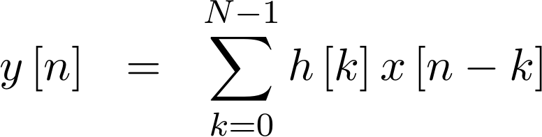Pictorially, this equation describes the operation shown in Fig 1 above.

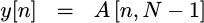
Today’s filter implementation will follow directly from a straight-forward evaluation of the summation in the equation above. In other words, we’ll start by setting an accumulator to the first value,

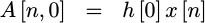Then, on each subsequent clock we’ll add the next value to it,

Fig 2. A Time Multiplexed filter implementation

Fig 2 on the right shows a diagram of how this approach might look. Basically, at every step we’ll read both an h[k] value and an x[n-k] value from separate memories, multiply the two together, and add the product together with the value from an accumulator. Once all the values have been added together, we’ll use this accumulated result as our output.

In Verilog, this might look something like the following. On the first clock, we’d read one tap from the tap (coefficient) memory, and multiply it by our incoming data sample, i_sample. The result of that product could then be used to initialize an accumulator, r_acc.

always @(posedge i_clk)
if (i_ce)
begin
	// first clock
	tap <= tapmem[0];

	// second clock
	product <= tap * i_sample;

	// third clock
	r_acc <= product;

Sounds simple so far, right? Okay, so we’ve ignored any pipeline scheduling (i_ce will only be true for one clock in N), but let’s come back to that in a moment.

Further, we’re going to need to read from block RAM memory on every clock following. This means we’ll need to place this new sample value into memory, and then increment the write pointer.

	// Write the new data to memory, then increment the memory pointer
	dmem[dwidx] <= i_sample;
	dwidx <= dwidx + 1'b1;	// increment the memory write pointer

We’re also going to want to be able to read the coefficient index pointer and the data index pointer on the next clock, so let’s set these as part of the same clock that the new data shows in on.

	// Still on i_ce
	tidx <= 1;
	didx <= dwidx;

After the accumulator has been given an initial value, we’ll then need to read both the coefficient values and the data values from an on-chip block RAM memory. Placing the data into a data memory to make this happen will require a memory write and some memory address manipulation. That means that the second part of this algorithm might look like:

end else if (!done)
begin
	// Now, between clocks, we'll need to read the data and the coefficient
	data <= dmem[didx];	// Read data from the sample memory, x[n-k]
	tap <= tapmem[tidx];	// Read from the coefficient memory, h[k]

	// Update the pointers to each.  Notice that the coefficient index,
	// tidx increases while the data index decreases--just as we have
	// above.
	didx <= didx - 1'b1;
	tidx <= tidx + 1'b1;

	// and calculate the product
	product <= tap * data;

	// Use the product to update the accumulator
	r_acc <= r_acc + product

Once we are done with all of the above, we’ll set the traveling CE values associated with the output, o_ce, and set the output value according to the last r_acc value.

end else // if (done)
begin
	o_ce <= 1'b1;
	o_result <= r_acc;
end

That’s the general gist of what we need to do. Sadly, however, the code above has multiple timing errors and pipeline scheduling conflicts within it. For example, there should be a clock delay between reading from memory and using the result, and another clock delay between multiplying two numbers together and using that result. As a result, the logic above will never work, but as a simple first draft it should be able to convey (roughly) what it is we hope to do.

The basic filter, written in C++

Perhaps if you have a software background, you might appreciate seeing this code written out in C++. The following is an excerpt from an FIR implementation found in my own personal signal processing library. The code uses double’s instead of fixed point, but it’s still basically the same thing.

This C++ algorithm depends upon an array of m_len coefficients, m_coeff. This array will be initialized with the coefficients associated with the filter before starting.

It also needs an array of data, m_data, of the same length. Rather than moving all the data through the array at every point in time, we’ll just keep track of the address of the last data element in the tapped delay line, m_loc.

class	FIR {
	int	m_len;	// Number of taps in the filter
	double	*m_coeff;

	// ...
	int	m_loc;		// Location of the last sample in the buffer
	double	*m_data;	// Data buffer, double[m_len]

	// ...
	// Declare our operator
	double	apply(double i_sample);
};

Were this written in Verilog, such as we will do in the next section, these two arrays would be captured in block RAMs.

To evaluate the convolution via the equation above, we’ll run the following code when given a new sample, i_sample.

double	FIR::apply(double i_sample) {
	int             i, ln;
	double  acc, *d, *c;

Our first step will be to record the new sample into the data memory.

	m_data[m_loc++] = dat;
	if (m_loc >= m_len)
		m_loc = 0;

After this point, we’ll enter a loop whereby we grab one sample from data memory and one coefficient from the coefficient memory, multiply the two together, and accumulate the result into an accumulator, acc. We’ll start the accumulator at zero. Further, after each sample, we’ll increase the address in coefficient memory, and decrease the address in data memory–just as the formula above indicated.

	acc = 0.0;
	d   = &m_data[m_loc-1];
	c   = &m_coeff[0];
	ln  = m_loc;
	for(i=0; i<ln; i++)
		acc += *c++ * *d--;

The fact that the data memory isn’t centered makes this a touch more complicated. What that means is that if you start reading backwards from the middle of memory (where the most recent sample was), you will eventually run off the beginning of the memory. Fig 3 shows this below.

Fig 3. Data memory contains both old and new data

In this figure, you can see the location m_loc (just right of the center of the figure) which is one past where the new data, i_sample, has just been written. You can also see how the x[n-k] sequence extends to the left of this location. Once this data sequence runs off the end of memory to the left, a second pass is required to get the rest of the data coming from the far end on the right. This second pass continues back to where we started, making sure every data sample in memory, and every coefficient value, is used exactly once.

	d   = m_data[m_len-1];
	ln  = ln-m_loc;
	for(i=0; i<ln; i++)
		acc += *c++ * *d--;

Once all of the multiplies have been completed, the result is returned.

	return acc;
}

This is the basic algorithm we will write in Verilog below. There will be some differences though. The first and most obvious difference is the fact that several parts of this algorithm will run in parallel–this is running in hardware after all. The next, not quite so obvious difference, is that if the memory address is limited to some finite number of bits, then we won’t need to pay any attention to the memory break shown above in Fig 3. Finally, the filter algorithm implemented in Verilog will be written using fixed point numbers instead of the double-precision floating point numbers that are so easy to use in the C++ above.

Before moving on, I should make one point about the code above. This C/C++ filter implementation is only practical for filters with impulse responses shorter than about 64 samples. Anything more than 64 samples and you’ll want to use an FFT based filtering approach. The differences between the two approaches will become particularly stark after doubling the filter length only a few times.

Verilog

Fig 4. Test Harness Filter Interface

You may remember from our test harness discussion that as long as a filter implementation has the ports we discussed then, and shown again here in Fig 4 at the right, that we can continue using our generic filtering test harness. While we’ll be able to inherit and modify the test harness with additional functionality in the next section, we’ll need to start out this section by remembering that our filter implementation will need to have a reset, and the ability to load taps, in addition to samples coming in and going out.

We’ll start with the ability to set our filter coefficients. As with many of our other filters, we’ll allow a parameter FIXED_TAPS to express whether or not this filter has a tap-update capability at all. If the coefficients are fixed, then we’ll $readmemh them from a .hex file whose name is given in INITIAL_COEFFS.

	generate if (FIXED_TAPS)
	begin
		initial $readmemh(INITIAL_COEFFS, tapmem);
		// ...
	end else begin

On the other hand, if our filter coefficients are not fixed, FIXED_TAPS will be false, and we’ll need to load our coefficients into memory. To do this, we’ll start with a memory index, tapwidx, or tap writing index.

		reg	[(LGNTAPS-1):0]	tapwidx;

We’ll set this index to zero initially, and to return to zero upon any reset.

		initial	tapwidx = 0;
		always @(posedge i_clk)
			if(i_reset)
				tapwidx <= 0;

Otherwise, anytime the i_tap_wr signal is high, a new coefficient is present in i_tap which we’ll write to coefficient memory. We’ll also need to increment this index.

			else if (i_tap_wr)
				tapwidx <= tapwidx + 1'b1;

Here’s where we actually use the tap (coefficient) writing index, tapwidx to write into the coefficient memory, tapmem. This is also the section of the code to specify any memory initialization, so we’ll initialize the memory if the INITIAL_COEFFS file name is empty. Note that the if statement is outside of the initial block. That will keep the synthesizer from looking for this file if the name hasn’t been given.

		if (INITIAL_COEFFS != 0)
			initial $readmemh(INITIAL_COEFFS, tapmem);
		always @(posedge i_clk)
			if (i_tap_wr)
				tapmem[tapwidx] <= i_tap;
	end endgenerate

That’s all that’s required for dynamically setting or adjusting coefficient memory. We started with an i_reset signal to clear the index, and then wrote one coefficient and stepped the index on any clock where i_tap_wr was true.

So let’s now turn our attention to the filter implementation itself.

We’ll start with updating the data memory, herein called dmem. We’ll use a data memory write index, dwidx to do this. Hence, on every i_ce value, we’ll increment the data memory write index,

	initial	dwidx = 0;
	always @(posedge i_clk)
		if (i_ce)
			dwidx <= dwidx + 1'b1;

and write the new sample into the data memory.

	always @(posedge i_clk)
		if (i_ce)
			dmem[dwidx] <= i_sample;

That may be about as simple as any logic could get!

That said, there is a subtlety associated with this approach. Notice in this process how the data memory update process is independent of the i_reset signal. It is dependent upon new sample data only. Further, this will allow the filter to immediately start with valid data following any reset.

This feature, however, will become a thorn in our side when we build our test bench. The basic problem is that we’ll want to apply test vectors to the filter that assume the memory is clear (all zeros). While the preferred solution might be to clear all memory elements any time i_reset is asserted, this isn’t how most memories are built. That means that, when we wish to clear this memory later, we’ll need to write as many zeros to it as are necessary to fill it with zeros.

Those two parts, loading tap coefficients and incoming data, are the easy parts of the algorithm, though. The next step is to calculate the indices to be used for both reading from coefficient and data memories. Since this gets into scheduling, let’s take a moment to start scribbling a draft pipeline schedule.

Usually, when I build a pipeline schedule, I start by writing out my code and marking each line with the appropriate clock. Doing this might result in pseudocode looking something like the following.

The first clock would set the memory read indices.

	// Clock 1 -- i_ce and i_sample are true, tidx and didx are set
	if (i_ce)
	begin
		tidx <= 0;
		didx <= dwidx;
	end else begin
		tidx <= tidx + 1'b1;
		didx <= didx - 1'b1;
	end

Notice how we are using the i_ce signal as an indication of when to reset the indices for the data and coefficient memories, didx and tidx, to the beginning of our run. At the same time, we’ll write the new data sample into memory–we discussed that above. That’s the first clock.

The second clock would read from memory,

	// Clock 2.
	tap <= tapmem[tidx];
	data <= dmem[didx];

This will give us the information we need to calculate h[k][x[n-k], hence we can multiply these two values together on the third clock cycle,

	// Clock 3.
	product <= tap * data;

Once the product is available, we’d add it to our accumulator.

	// Clock 4.
	if (new_product_data)
		acc <= product;
	else if (subsequent_product_data)
		acc <= acc + product;

The final step would be to create our output. This will need to take place some time into the future–at a time we’ll need to come back to and determine later.

	// Clock ... some distance into the future
	if (new_product_data)
	begin
		o_ce <= 1'b1;
		o_result <= acc;
	end else
		o_ce <= 1'b0;

Before moving on, I tried to draw this basic pipeline schedule out in Fig 5 below for reference. You should know, though, that whenever I build an algorithm like this I usually just start by writing the clock numbers in my code as we just did above. I find these diagrams, like Fig 5 below, are most useful to me when telling someone else about one of my designs, such as I am doing now, then they are when I write them.

Fig 5. Initial draft pipeline schedule

If you aren’t familiar with this sort of table, I use it to communicate when variables are valid within a design. In this case, on the clock that any new data is present, i.e. the clock where i_ce is high, the write index for the data memory will also be valid. These clock numbers are off by one from the ones above, simply because variables set on one clock (as shown in the code above) will be valid on the next clock–as shown in Fig 5.

So, that’s generally what we wish to do. To make this happen, though, let’s add some traveling valid flags to this pipeline. Specifically, we are going to want to know when to reset the accumulator with a new product, and when to add other products into the accumulator. We’re also going to need to know when to set o_ce and o_result.

The first traveling valid flag we’ll call pre_acc_ce–or the pre clock enable for the accumulator. We’ll use a shift register for this purpose. Hence, on the first clock we’ll set pre_acc_ce[0] to let us know that the indices will be valid on the next clock. On that next clock, we’ll set pre_acc_ce[1] to indicate that the memory reads are valid. Finally, we’ll set pre_acc_ce[2] to indicate that the product is valid. Further, we’ll clear pre_acc_ce[0] as soon as the last tap has been read. This will then be the indicator needed to know when to stop accumulating values.

The only real trick in this logic chain is knowing when to shut pre_acc_ce[0] off. In particular, it needs to be shut off once we have exhausted all of the coefficients in the filter. We’ll come back to this in a moment, but for now we are talking about a simple piece of scheduling logic such as,

	wire	last_tap_index;
	// ...
	reg	[2:0]	pre_acc_ce;
	initial	pre_acc_ce = 3'h0;
	always @(posedge i_clk)
		if (i_reset)
			pre_acc_ce[0] <= 1'b0;
		else if (i_ce)
			pre_acc_ce[0] <= 1'b1;
		else if ((pre_acc_ce[0])&&(last_tap_index))
			pre_acc_ce[0] <= 1'b1;
		else
			pre_acc_ce[0] <= 1'b0;
	// ...

	always @(posedge i_clk)
		if (i_reset)
			pre_acc_ce[2:1] <= 2'b0;
		else
			pre_acc_ce[2:1] <= pre_acc_ce[1:0];

Once i_ce is valid, the memory index will be valid on the next clock–so we’ll set pre_ce_acc[0] to true. We’ll leave it true until we get to the last tap index. Likewise the values will flow through this structure just like a shift register.

But when shall we cut it off? It needs to be cut off such that, when the coefficient index, tidx, is referencing the last coefficient, pre_acc_ce[0] will be false on the next clock. Since our coefficient index is counting from 0 to NTAPS-1, this can be expressed as,

	assign	last_tap_index = (NTAPS[LGNTAPS-1:0]-tidx <= 1);

The neat thing about this piece of logic, as you’ll see as we move forward, is that it keeps the filter from outputting an invalid answer any time too many clocks are given between i_ce values. Hence, if you have a filter with NTAPS coefficients, yet there are more than NTAPS clocks between samples, then the accumulator will only pay attention to the first NTAPS products.

This brings us to our next step: the block RAM read indices. Upon any new value, the filter starts accumulating from the product of coefficient zero and the most recent data sample. Coefficients then work forwards in their array, while the data indexes work backwards–just like they did in the convolution formula we started with.

	initial	didx = 0;
	initial	tidx = 0;
	always @(posedge i_clk)
		if (i_ce)
		begin
			didx <= dwidx;
			tidx <= 0;
		end else begin
			didx <= didx - 1'b1;
			tidx <= tidx + 1'b1;
		end

Indeed, this logic is essentially identical to our last draft.

We’ll also follow the clocks through the pipeline with a second traveling CE approach that will use a couple of other CE signals. The first of these, m_ce is memory index valid signal, indicating that the first indices is valid. As you follow through the code, you’ll see other similar CE signals, such as the d_ce signal to indicate the first set of data and coefficient values are valid and p_ce to indicate the first product is valid. We’ll use these in a moment to determine when to load the accumulator vs adding a new value to it.

	// m_ce is valid when the first index is valid
	initial	m_ce = 1'b0;
	always @(posedge i_clk)
		m_ce <= (i_ce)&&(!i_reset);

On every clock cycle, we’ll read two values from block RAM–a filter coefficient value and a data value. Note how the block RAM reading code below is explicitly kept very simple. This is to make certain that the tools recognize these as reads from block RAM’s, rather than more complex logic such as one would need to implement via a look-up-tables.

	initial	tap = 0;
	always @(posedge i_clk)
		tap <= tapmem[tidx[(LGNTAPS-1):0]];

	initial	data = 0;
	always @(posedge i_clk)
		data <= dmem[didx];

Once read, we’ll set a data CE, or d_ce, to indicate that the first data value is now valid. This will follow the first memory indices are valid CE, m_ce.

	initial	d_ce = 0;
	always @(posedge i_clk)
		d_ce <= (m_ce)&&(!i_reset);

After all this work, we can now calculate the product of h[k]x[n-k], herein referenced as just tap * data. Another traveling CE value, this time p_ce, denotes when this first product is valid.

	initial	p_ce = 1'b0;
	always @(posedge i_clk)
		p_ce <= (d_ce)&&(!i_reset);

	initial	product = 0;
	always @(posedge i_clk)
		product <= tap * data;

Only now can we can finally get to the accumulator at the penultimate stage of this chain. On the first value given to it, that is any time p_ce is true–which will be true with the first product value, h[0]x[n], the accumulator is set to the result of that first product. Otherwise, any time a subsequent product is valid–as noted by pre_acc_ce[2] being high, the accumulator value is increased by that clock’s h[k]x[n-k] value.

	initial	r_acc = 0;
	always @(posedge i_clk)
		if (p_ce)
			r_acc <={ {(OW-(IW+TW)){product[(IW+TW-1)]}}, product };
		else if (pre_acc_ce[2])
			r_acc <= r_acc + { {(OW-(IW+TW)){product[(IW+TW-1)]}},
						product };

This almost looks like the draft code we created to work out pipeline scheduling. The biggest difference is that we’ve done some sign extension work above to make sure this works across multiple synthesis tools and lint checkers.

On the same clock we place a new value into the accumulator, we can also read the last value out. Hence we set o_result to the output of the accumulator on that same clock, and o_ce to indicate this result is valid.

	initial	o_result = 0;
	always @(posedge i_clk)
		if (p_ce)
			o_result <= r_acc;

	initial	o_ce = 1'b0;
	always @(posedge i_clk)
		o_ce <= (p_ce)&&(!i_reset);
endmodule

Note that, as a consequence of this approach, o_ce will always be true a fixed number of clock ticks from i_ce. Hence, if the data stops coming, the last accumulator value will not be read out. Likewise, if the i_ce values come with fewer than NTAPS steps between them, then the o_ce values will only report partial filter products. There is no error detection or correction here–but you can feel free to add it if you would like.

Still, that’s what it takes to generate a slow FIR filter in Verilog for an FPGA. Sadly, though, the code is complex enough that we are going to lean heavily on our test bench code to know if it works or not.

Test bench

When it comes time to building a test bench for this filter, we’ve really already done most of the work in the generic filtering test harness we built for the generic filter’s test bench. As a result, testing this filter only requires making a couple of small changes. Indeed, if you run a diff between the original test bench for a generic filter and the test bench for this filter, you’ll see the changes we are about to discuss below. You might even be surprised at how much code is in common between the two.

This will, however, be the first filter that will test the fixed number of clocks per input clock enable, i_ce associated with the sample value. As it turns out, we did a good job building the initial test harness, so there’s not much that needs to be changed there.

Second, unlike the prior filter, resetting this one so that all the memory is zero requires more work than just setting the reset flag. In particular, the way block RAM’s are built, they cannot be cleared in a single clock. As a result, we’ll need to write a routine to explicitly write zero samples to the filter’s internal memory so that any test vector generator can start from a known state.

With those two caveats aside, let’s start looking at the code.

As with any code using our basic filtering test bench, it starts out be declaring constants shared between the test bench code and the filter itself. These include the number of bits in the input, the coefficients, the output, the number of coefficients, the delay between input and the first output resulting from that input, and the number of clocks per input sample.

const	unsigned IW = 16,
		TW = 16,
		OW = IW+TW+7,
		NTAPS = 110,
		DELAY = 2,
		CKPCE = NTAPS;

These values are not only declared as constants at the beginning of the test bench, but they are also used to when initializing our test bench class.

class	SLOWFIL_TB : public FILTERTB<Vslowfil> {
public:
	bool		m_done;

	SLOWFIL_TB(void) {
		IW(::IW);
		TW(::TW);
		OW(::OW);
		NTAPS(::NTAPS);
		DELAY(::DELAY);
		CKPCE(::CKPCE);
	}

This is just normal setup though. Now we need to get into the actual details of the test bench changes.

The first change that needs to be made is to the test() routine. This routine, as you may remember, takes an input data stream, applies the filter, and returns the result. It also depends upon the filter having a zero internal state. Since clearing the state in this test bench is a little more awkward, we’ll make certain to call a function to make certain the state is cleared before calling the test() function in the test harness itself. The neat part of this change, though, is that by overloading, this test() operator and using inheritance, this change only requires the following four lines of code.

	void	test(int nlen, long *data) {
		clear_filter();
		FILTERTB<Vslowfil>::test(nlen, data);
	}

Unlike the other filters we’ve tested, this one requires a reset prior to loading any new coefficients. As you may recall from above, resetting this filter sets the index into the coefficient memory back to zero, so it is an important part of loading a new set of coefficients. Just a slight modification to the test bench, and this change has now been made as well.

	void	load(int nlen, long *data) {
		reset();
		FILTERTB<Vslowfil>::load(nlen, data);
	}

Perhaps the most important change, though, is the function that we need to write to clear the data memory within this filter. We’ll call this function clear_filter(). It will work by providing one clock with i_ce high and i_sample set to zero per element in the memory array. Since the array will always be a length given by a power of two, the internal memory may also be longer than the number of taps, NTAPS() in this filter. For this reason, we’ll round up to the next power of two using nextlg().

What may surprise you, though, is that we are going to hit this filter with one new sample per clock, while ignoring the output. The result of this will be that the output of this run will be invalid, although the new data will loaded into he memory as desired.

	void	clear_filter(void) {
		m_core->i_tap_wr = 0;

		// ..
		m_core->i_ce     = 1;
		m_core->i_sample = 0;
		for(int k=0; k<nextlg(NTAPS()); k++)
			tick();

As one final step, once the memory has been loaded, we’ll let the last sample propagate through the filter, so as to make certain the filter is in a usable state when we apply our test vectors.

		m_core->i_ce = 0;
		for(int k=0; k<CKPCE(); k++)
			tick();
	}
};

At this point, all we need to do is switch our main program to running the test bench created for this new code, and everything is roughly the same as before.

SLOWFIL_TB	*tb;

int	main(int argc, char **argv) {
	Verilated::commandArgs(argc, argv);
	tb = new SLOWFIL_TB();

How’s that for fairly simple? Indeed, implementing the filter itself was harder than this test bench.

Of course, it’s only that simple because of the work we’ve already done, but that just underscores the power of Object Oriented Programming (OOP).

Example Traces

If you’d like to see a trace of how this all works, there’s a commented line in the test bench,

	// tb->opentrace("trace.vcd");

which, if uncommented, will create a VCD file containing a trace of what this filter does in response to the test bench’s stimulus. Be careful–the trace can quickly become hundreds of megabytes, if not several gigabytes, in length.

Still, let’s turn that on to see if we can get a feel for how this filter works. We’ll stop the test bench after the trace file gets to about 28MB–which is still more than we need for this demo. We can then use GTKwave to display the results. You can see a screen capture of the result in Fig 6 below.

Fig 6. Trace of the First Impulse Test

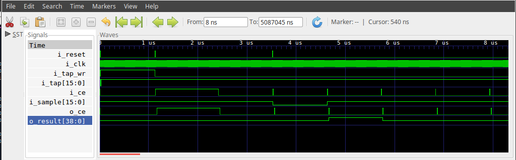The figure shows several key steps in the test bench.

1. First, at the far left, i_tap_wr is high for many clocks as the coefficients (i_tap) are loaded into the filter.

2. The filter is then cleared by writing a series of (roughly) NTAPS() zeros into the memory.

3. The test bench then applies an impulse to the filter, to verify the response. Both impulse and coefficient value are negative maximums, to see if the filter will overflow as a result. What that means, though, is that the filter’s output given these coefficients and this input will be a single positive impulse, as shown in the figure above.

Suppose we zoomed in some more on how this filter operated? In this case, see Fig 7 below.

Fig 7. Zooming in on the first test vector

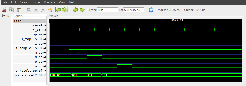At this zoom level, you can see how the various CEs (really misnamed valid signals) make their way through the system until the final o_ce and o_result are valid. You can also see the pre_acc_ce[2:0] shift register note when the tap index and data index became valid, m_ce, when the memory reads were valid, d_ce, and when the products became valid, p_ce.

The point here is, even if you are struggling to understand the code itself above, sometimes a trace becomes easier to make sense of.

Conclusions

This filtering approach is really quite powerful. Not only were we able to reduce the number of multiplies required in order to implement this filter, but we were also able to prove it using little more than the test harness code we’ve already built.

Remember the discussion we started out with regarding a 2047 tap filter? Such a filter would be sufficient to generate a lowpass filter with a 480Hz passband, a 176Hz transition band, and a 70dB stop band. That’s probably good enough for any audio work you might wish to do.

That doesn’t mean this is the best (or worst) filter out there, just one to place into your tool box. It has a purpose, and it works well in its own niche.

What other approaches might we have tried?

I’ve mentioned for some time that I’d like to build and demonstrate a symmetrical filter. At high speed, that filter is now built and just waiting for a good blog post. Similarly, a fun challenge might be to modify this filter to handle symmetric coefficients, something that would allow it to run twice as many coefficients at once.

Another future filter that will be fun to present is what I’m going to call a cascaded filter. By cascaded filter, I mean one that is basically identical to this filter, except that it allows multiple filters of this type to be cascaded together in order to effectively create a much longer filter. In many ways, this may seem like the holy grail of generic filter implementation–a filter that can be adjusted to use only as many hardware multiplies as it is required to use given the incoming data rate.

Perhaps the ultimate lowpass filter, however, is the multirate implementation of a lowpass filter. Using multirate techniques, it should be possible to apply a lowpass filter of any bandwidth to full speed data for a cost of only 10-12 multiplies.

But these are all topics for another day.