
Interpolation is just a special type of convolution
The most profound lessons I’ve learned regarding interpolation were that first, shift invariant interpolators existed, and second that the effects of a shift invariant interpolator can be described in the frequency domain.
But let’s back up a step to tell this story from the beginning.
Interpolation refers to a class of methods or algorithms for reconstructing a waveform’s value between given sample points. Interpolation is an important part of any sample rate conversion algorithm. As a result, it is studied as part of both numerical analysis is as well as mutirate digital signal processing.
As part of this blog, we’ve already discussed nearest-neighbour interpolation and linear interpolation. Going further, though, requires a bit of a background understanding. Since the necessary background wasn’t something I learned when I last studied numerical analysis, I figured you might be interested as well.
Today, therefore, let’s look beyond linear interpolation and lay the ground work for better FPGA based polynomial interpolation algorithms.
My own history with interpolation
I first became seriously interested in interpolation when I tried to follow and recreate William Gardner’s cyclostationary signal processing results as part of my Ph.D. Research. Gardner had stated that by using cyclostationary methods, his time difference of arrival (TDOA) algorithm could outperform all others.
These new algorithms are tolerant to both interfering signals and noise, and they can outperform conventional algorithms that achieve the Cramer-Rao lower bound on variance for stationary signals because the signals considered here are nonstationary (cyclostationary) and the algorithms expoit the nonstationarity to discriminate against noise and interference.
A TDOA estimator, for those not familiar with the algorithm, takes two input signals, where one is nominally the other delayed by some amount of time, runs a cross-correlation between them, and then finds the location of the maximum value that results. [Ref]
Gardner, however, had insisted in his problem setup that the two simulated signals were to be delayed with respect to each other by an integer number of samples, and then assumed the peak would lie on a sample point. This process skipped the interpolator that would be necessary for any real life application, and so his estimation errors suddenly (and artificially) dropped to zero. This erroneous result then overinflated the performance of his algorithm.
This lead me to study the question of which interpolator is better when peak finding?
Peak finding in TDOA estimation, however, is only one purpose of an interpolator. Other purposes for interpolation aren’t hard to come by:
-
Interpolators are commonly needed to process audio signals. They are used to change sampling rates, such as from an 8kHz sample rate to a 44.1kHz sample rate, or from a 44.1kHz sample rate to a 48kHz sample rate.
-
Interpolators are used within video display devices having a fixed resolution, to allow them to display other resolutions.
-
When I was working with GPS signals years ago, the digitizer would sample some integer number of samples per chip. However, in order to use Fast Fourier transform signal processing methods, the data needs to be resampled from the 1023N samples per block that came from the digitizer to
1024*2^Msamples per block–a power of two. This requires an upsampling interpolation rate of 1024/1023—a difficult ratio to achieve using rational resampling methods. (In the end, we actually downsampled the signal by 8192/1023 …)Indeed, interpolation in a GPS processing system isn’t limited to the front end (re)sampler. It’s also an important part of picking the correlation peak that is part of the measurement used to determine your location as well.
-
Many sine wave implementations are based around a table lookup. If you want to control the distortion in the resulting sine wave, knowing how the interpolator responds is important to evaluating how good your table lookup method is.
-
Most satellite orbits are communicated with sampled positions from a special orbital propagator. However, satellite navigation work, such as GPS, requires knowing the satellite’s position often on nanosecond level timesteps. Interpolation is used to address the problem of determining what happens between the points.
Even better, as we’ll touch on below, if you can quantify the error in your interpolator, such as by using Fourier analysis, you can also quantify the error in your navigation system. You might even be able to relax the requirements of your numerical satellite propagation engine with a sufficiently powerful interpolator.
-
When I built a suite of tools for digital signal processing and display years ago, I used an interpolator as part of the GUI to allow the user to zoom in on any signal by an arbitrary amount. Even better, by using a quadratic interpolator, the signal lost most of the obvious evidences of being sampled in the first place.
-
When presenting the demonstration of the improved PWM signal, we only used a nearest-neighbour interpolator to go from the audio sample rate to output samples. Because we didn’t use a good interpolator, our test waveform had many aliasing artifacts in addition to the artifacts due to the PWM modulation.
Replacing the nearest-neighbour interpolator with either a linear or quadratic interpolator would’ve removed most of those extra artifacts.
While the description above highlights my own personal background and reasons for studying interpolation theory after my graduate studies, these few examples can hardly do justice to the number of times and places where a good interpolator is required. Hence, when it comes time for you to choose a good interpolator, you’ll want to remember the lessons we are about to discuss.
Key Assumptions
The field of interpolation is fairly well established with lots of approaches and “solutions”. To limit our discussion, therefore, we’ll need to make some assumptions about what types of interpolators are appropriate for signal processing on an FPGA. You may wish to read this section carefully, though, because the interpolation theory and conclusions I’ll present later will be driven by these assumptions.
The first couple of assumptions are quite basic to digital signal processing in general: the input is assumed to be a sampled data stream that is formed from sampling: an infinite signal source (in time) at equidistant samples. An example of such a sampled signal is shown below in Fig 1.
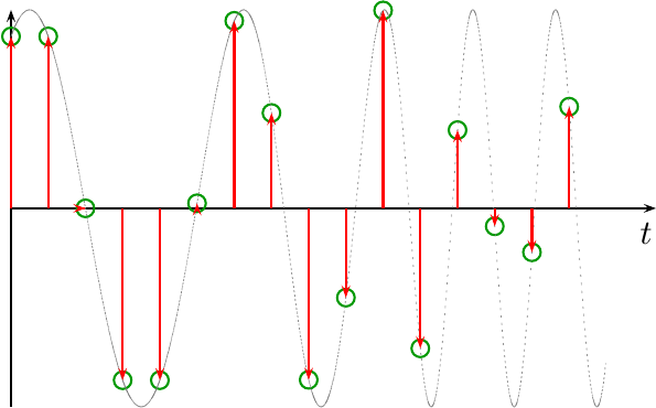 |
In the figure above, you can see the sampled points represented by green circles, and the original waveform in dotted gray. The purpose of the interpolator is to estimate or recover the signal between the sample points.
The waveform shown in Fig 1 above also makes a wonderful example waveform: it is a swept frequency tone. Hence, the frequency of the tone on the left is lower than that on the right. As a result, and as we’ll discuss, interpolating the signal on the left side is easy, but it gets harder on the right. Indeed, you might notice within the figure how aliasing starts to dominate on the far right. Indeed, this figure works as such a good interpolation test, that I used it throughout the tutorial slides I built to discuss this the topic. We can return to this later.
For now, let’s introduce two further key assumptions.
-
The first of these key assumptions is that we are looking for a linear operator. Adding two sample streams together before applying the interpolator should therefore produce an interpolation of their sum signal. Multiplying the incoming signal by a constant (scalar) should produce a scaled output signal.
While quantization will have an effect on these two properties of linearity, let’s ignore it for now and just focus on interpolating real signals.
-
The second and final key assumption is that that the interpolation approach we are interested in today is shift invariant. Shift invariance in this case is a subtly different from the classic definition simply because the input is a sampled data stream, defined over the domain of all integers, and the output is a signal defined over the domain of real numbers. Therefore, by shift invariant I mean that if you shift the incoming sample stream left or right by some integer number of samples,
k, then the interpolated output stream (defined over the domain of real numbers) will also shift by the same integer amount.
That’s not so hard, is it?
The goal of any interpolation algorithm is to estimate or recover the signal between the sample points. If you think about interpolation in terms of Fig 1 above, the goal is to recover the gray dotted line given only the green points.
The above assumptions also drive the form of the interpolation solution.
To see how this is the case, let’s start with a mathematical representation of
our sampled
signal, x[n], re-expressed as a series of
Dirac delta functions
over the
domain
of real numbers.
![x(t)=SUM x[n]d(t-n)](/img/interp-x-made-continuous.png) |
In this representation, the function x(t) is created from the discrete-time
input sequence x[n] by a sum of scaled and offset
Dirac delta functions.
Indeed, this was the meaning of the red impulses shown in Fig 1 above. Each
impulse
represents a scaled
Dirac delta function,
at the
sample
height, x[n], and location, n, just as this equation describes. These
Dirac delta functions
are used to bridge the difference between the
sampled
representation of a signal, x[n], and its continuous time equivalent,
x(t).
We also know that every
linear
time-invariant system
producing an output y(t) from its input x(t) can be represented by a
continuous-time
convolution, such as the one
shown below.
 |
At this point in our discussion, the form of the h(t) that describes this
system is completely arbitrary. It’s just a function of the
real numbers, producing a
real numbered output. We’ll
come back later and pick a particular form to work with, but for now consider
h(t) to be an arbitrary
real
valued function.
Since we’ve represented our original
sampled
signal, x[n], with a representation, x(t), composed of a set of scaled and
offset
Dirac delta functions,
we can then substitute x(t)
into this formula,
![y(t)=INT h(tau) SUM x[n] d(t-tau-n)](/img/interp-xn-convolved.png) |
and then pull the summation out front,
![y(t)=SUM x[n] INT h(tau) d(t-tau-n)](/img/interp-xn-convolved-2.png) |
The result is a convolution that we can evaluate. Given the properties of the Dirac delta functions, any product of a Dirac delta functions and a function that is continuous near the region where the Dirac delta functions is non-zero, yet integrated over the point where the argument of the Dirac delta functions is goes through zero will simply yield the value of that other function at that point. In other words,
![y(t)=SUM x[n] INT h(tau) d(t-tau-n)](/img/interp-is-convolution.png) |
and we’ve just proved that, under the assumptions we listed above, interpolation is just another form of a convolution.
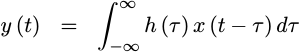
To see what I mean by this, consider Fig 2 below.
 |
In this figure, you can see the operation of the
convolution
taking place. The figure shows the incoming
samples,
as green dots. For each incoming
sample,
there is a scaled and weighted h(t) function shown in gray. Note how
this h(t) function was designed so that the each gray line touches one
green circle, and yet goes through zero for the other circles. Then, when
you sum all of these weighted and shifted h(t) functions together, you get
the interpolation
result shown in red.
This conclusion has some major consequences for signal processing. Among other things, it means we can use Fourier analysis techniques to evaluate interpolators–just as we use Fourier analysis to evaluate any other filtering operation.
In particular, we can treat an interpolator as nothing more than an upsampling filter. Everything you’ve learned about aliasing and Nyquist sampling applies now as it would with any other upsampling filter.
Sadly, apart from the modern development of Farrow filters, it seems that only a few interpolation developments start from these assumptions. We’ll discuss the consequences of other choices quickly in the next section.
Without loss of (too much) generality, we can use a
piecewise
polynomial
to represent the h(t) function above. Doing so allows us to turn our
incoming
sampled
signal, x[n], into a
piecewise
polynomial, y(t), meaning
that what happens between
samples, i.e. the
interpolator
result, can now be represented as a
piecewise
polynomial.
Two piecewise
polynomial
forms are convenient for this purpose: those centered around the points
where the signal is defined, [k-0.5,k+0.5) for
integers
k, and those defined between points
in a signal, such as [k, k+1). We’ll come back to this more in a moment.
So, to summarize, here were our assumptions:
-
The incoming signal was sampled
This will be the case with almost all DSP applications.
-
The incoming signal is infinite in length.
While one might argue that this is never quite true, it is true that for most signal processing applications there is often more data available than can be operated on at any point in time. For these applications, the difference between a signal of truly infinite length and the perspective of the signal processing engine applied to a signal of finite length is quite irrelevant.
-
All sample times are equidistant
This is also true for most, although not all, DSP applications.
-
The interpolator must be linear.
-
The resulting interpolator must also be shift invariant
This may be the most significant assumption we’ve made along the way. Indeed, it is this assumption that renders most of the other interpolation developments inappropriate going forward–since they don’t preserve this property.
It is also this assumption that makes Fourier analysis of the interpolator possible.
-
The interpolator’s interpolation function,
h(t), is formed from a set of piecewise polynomials.I’m sure there must be other useful interpolation functions that are not formed from piecewise polynomials. However, piecewise polynomials form a nice, easy set to work with when implementing interpolators within FPGAs–or even embedded CPUs for that matter.
For the most part, these are all quite common digital signal processing assumptions, so I wouldn’t expect anyone to be surprised or shocked at any of them. What has surprised me was how rare these assumptions are in the interpolation developments I’ve studied in the past.
Many other approaches are not shift invariant
Since the assumptions above are not common interpolation assumptions, let’s take a moment and investigate the significance of some of them.
Traditional interpolation approaches are commonly applied to only a finite set of sample points found within a single, fixed, finite window of time. This includes most spline interpolation developments (these were always my favorites), Chebyshev polynomial interpolation, Lagrange interpolation, Legendre polynomial interpolation and more.
These approaches, however, become less than ideal when applied to a sample stream that is much longer than their finite time window. Therefore, to make these approaches viable, the sample data stream is split into windows in time and the interpolator is applied to each window.
The problem with this sliding window approach revolves around what happens at the edges where the algorithm transitions from one window to the next. Because these interpolation routines do nothing to guarantee that the result has controlled properties between one window and the next, the transition region often suffers from distortions not present in the interpolator’s development.
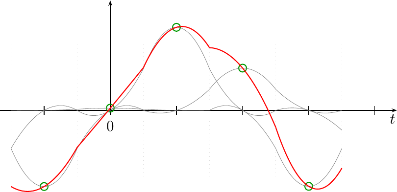
Nowhere is this more apparent than when combining a series of quadratic fits between sample points together to create a new interpolated signal, such as is shown in Fig 3.
 |
In this figure, every set of three adjacent sample points was used to create a quadratic interpolation function surrounding the middle sample. The interpolation function is only valid for plus or minus a half sample surrounding the middle of those three points. Outside of that region, a new set of three samples is used to generate the next quadratic fit. The resulting signal, shown in Fig 3 above, contains many unwanted discontinuities that result from this sliding fit-window approach.
Further, our desire to create an interpolation filter that can be implemented within an FPGA will tend to push us away from other common filter structures, such as trigonometric interpolation, or even rational function evaluation, since these interpolators depend upon functions that are more difficult to calculate within RTL logic. That leaves us stuck with piecewise polynomial interpolation functions.
Not all of the other approaches avoid
shift invariance.
For example, the Whittaker-Shannon
interpolation
approach creates a
shift invariant
interpolator
that can be applied to the infinite sample sets discussed above. However, the
sinc functions
it is based upon an h(t) that is infinite in length, making this approach
difficult to implement.
As a result, this leaves us with only one practical interpolator choice, which we shall discuss in the next section.
Farrow Filters
The only viable interpolation alternative remaining within this set of assumptions is a Farrow filter. Indeed, the assumptions we’ve arrived at so far force us towards a Farrow filter, leaving us no other alternative.
 |
When using the Farrow filter
approach, the
interpolation
function, h(t), is formed from a set of
piecewise
polynomials. An example of one
such filter composed of
piecewise
quadratics
is shown in Fig 4 on the right.
According to
Farrow’s paper, the actual
“amount of delay”, i.e. the t value when calculating the
interpolation
result, need not be calculated until it is needed. This
is perfect for what we might wish to accomplish within an
FPGA.
The only question remaining is, what
interpolation
function, h(t), shall we use?
Fred Harris presents a solution to interpolation function generation based upon first designing a discrete-time filter of many taps, and then approximating that function with a higher order polynomial. You may find this approach a valid solution to your interpolation needs. It is actually commonly used.
I just haven’t found Harris’s ad-hoc filter derivation method personally very satisfying. Ever since finding Harris’s work, I’ve wanted to know if there were a more rigorous and less ad-hoc approach to generating these coefficients. Is there some way, therefore, that an interpolator can be developed using this technique and yet still meeting some optimality properties?
The answer is, yes there is, but also that we won’t get that far today. Instead, we’ll just lay the ground work for understanding and analyzing filters of this type. Then, later, we’ll use this approach in order to develop optimal (in some sense) interpolation functions and their piecewise polynomial coefficients.
Some example filters
For now, let’s demonstrate some example Farrow filters. Our examples will have a much lower order than those either Farrow or Harris used, but the lower order might help to make these filters more understandable.
Sample and hold
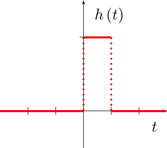 |
The first interpolator we discussed on this blog was a sample and hold function. While this may not seem like much of an interpolator, it can be shown to have the form shown in Fig 5 on the right, and in the equation below:
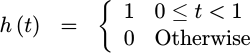 |
This is actually a common interpolation function in many mixed signal components, so it is worth recognizing.
While this a common interpolation function in many practical mixed signal components, I’d like to do better. Let’s keep looking, therefore.
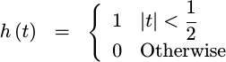
Nearest Neighbour
A similar interpolation
function is the
nearest neighbor
function. This has
an almost identical form for h(t) as the sample-and-hold function above,
save that this time h(t) is centered about the y-axis.
 |
It isn’t all that difficult to prove that the
Fourier
transform of this function is a familiar
sinc function, which decays
out of band at a rate of 1/f. Fig 6 below shows both this h(t) function,
on the left, as well as its
frequency response
on the right. Also shown on the
frequency response
chart is a 1/f asymptote.
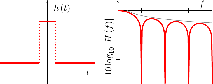 |
The asymptotic performance can be controlled in filter design to achieve specific performance measures, if desired. You’ll be able to see this as we continue.
Linear interpolation
If you convolve the rectangle function that is the nearest neighbor interpolator with itself, you will get a triangle functions,
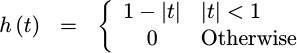 |
Since convolution in time is multiplication in frequency, the Fourier transform of this function is simply a sinc function squared.
 |
This creates a 1/f^2 asymptote, shown above. As a result, any out of band
aliasing
artifacts are further attenuated by this filter.
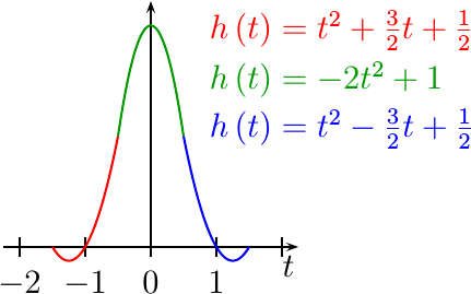
Quadratic Fit
With a little bit of work, the typical quadratic fit function, the one producing the result in Fig 3 above, can also be represented in this form.
 |
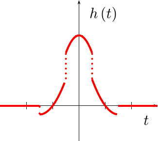 |
This function, however, isn’t continuous at all. Indeed, when you plot it out, as in Fig 8 to the right, you’ll get a feel for why the quadratic fit in Fig 3 above looked as horrible as it did.
But, what happened? Why does this look nothing like a quadratic fit?
Well, actually, it does. If you extend the middle section on both sides,
you can see that it comes down and hits the axis at x=-1 and x=1. In
a similar fashion, if you extend either of the wings out, you’ll see they
hit y(0)=1 and either y(-2)=0 or y(2)=0 respectively. We created
exactly what we tried to create, but by moving from one fitting window
to the next we also created the discontinuous artifacts shown in Fig 8.
This really shouldn’t be surprising. When we created our quadratic fit, we did nothing to control the transitions from one fitting region to another. Fig 8 just shows the effects of such a choice on the filter that results.
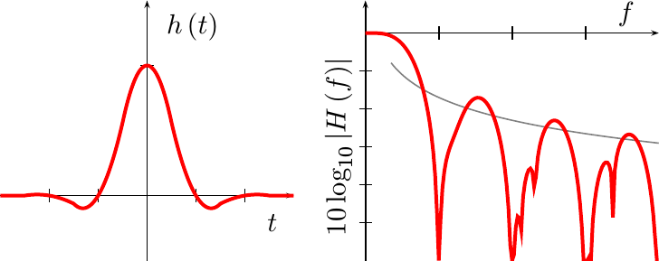
Smoothed quadratic
If convolving
a rectangle
with itself generated a nice linear
interpolation
triangle function,
what do you think you would you get from
convolving a
triangle function
with that same
rectangle? You will
get a
piecewise
quadratic
polynomial
function whose
frequency response
decays at 1/f^3–as fast or faster than any other
piecewise
quadratic
polynomial
function.
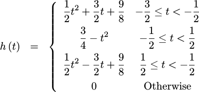 |
The only problem with this function is that it is no longer a true
interpolator.
By that I mean that if you were to
convolve
your sampled data, x[n], with this function, then the continuous output
function, y(t), that would result would no longer necessarily match
x[n] whenever t=n.
This is a result of the fact that h(n) doesn’t equal zero for all
integers, n, where n != 0.
You can see from Fig 9 below that this
function certainly doesn’t go through zero at t=1 as just one example.
 |
The good news, though, is that the 1/f^3 falloff was one of the best we’ve
seen yet–as shown by the
frequency response
function on the right of Fig 9 above.
Since we are trying to create interpolators, a function that isn’t an interpolator isn’t very acceptable. Therefore let’s remember this function while looking for an better alternative.
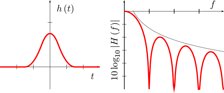
Ideal Interpolator
 |
Much as it is possible with traditional filtering methods to specify an ideal filter, the same can be done with interpolation filters as well.
Shown in Fig 10 at the right is the frequency response of an ideal interpolation filter. As you might expect, this function passes all frequencies below the Nyquist frequency, and stops all frequencies above that.
However, as with the development of more traditional filters, this interpolator is also infinite in length, doesn’t fit nicely into a piecewise polynomial representation, and thus isn’t very suitable for practical work.
It is suitable, however, for discussing the ideal that we would like our practical filters to approach in terms of performance. Therefore, we shall judge that the closer an interpolation filter’s frequency response approximates this ideal filter, the better the interpolation will be.
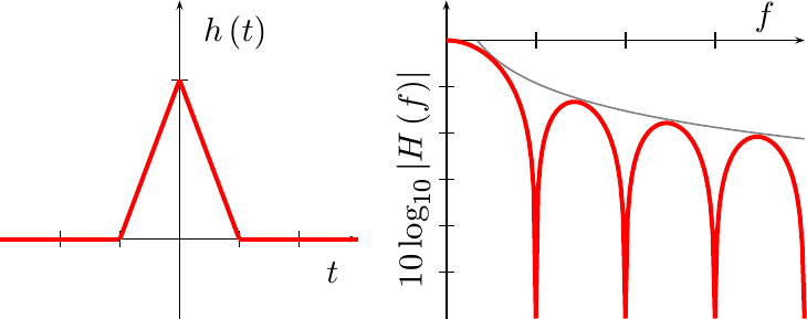
Better Quadratic
With a bit more work, we can come up with a better quadratic
interpolation
function. This function, shown in Fig 11 below, has a much wider
“passband”,
while still maintaining the 1/f^2
stopband
fall off that the linear
interpolator had.
 |
Not only that, but this filter comes closer to the ideal in both passband and stopband then our last attempt did. Hence, while maintaining the asymptotic performance of a linear interpolator, we’ve achieved better performance at lower frequencies. Further, the nulls are deeper and wider than the linear interpolator shown in Fig 7 above.
For these reasons, this will be the filter we’ll implement and demonstrate when we come back and look at quadratic interpolation performance in a later post.
Can we do better?
I think the answer to this question is, yes, we can do even better than this. However, I have yet to see the formal theory behind optimally generating interpolation functions such as these.
For now, consider this question: can the ad-hoc
Farrow filter functions that
Harris espouses be
rewritten as discrete
convolutions
of functions which are formed by
convolving a
rectangle
rectangle with itself many times? If so, you could choose the rate at
which the stop band falls off, whether 1/f, 1/f^2, etc, by choosing
which subset of these functions you wish to use when generating your
interpolation
function.
Conclusion
Selecting a “good” interpolation method for your signal processing application starts with the right set of assumptions. Indeed, the single most critical assumption required for good interpolator development is that the resulting interpolation method must be shift invariant. Interpolation routines chosen without this property are likely to suffer uncontrolled effects as the interval defining the function changes with time.
This, however, is only the beginning of the study of interpolation for DSP applications within FPGAs. While it opens up the topic by providing the necessary background, more remains to be covered. For example:
-
It is possible, although perhaps not all that practical, to create a spline development under these assumptions. Although the typical spline development depends upon a difficult matrix inversion, an alternative spline development exists which doesn’t depend upon any real-time matrix inversion.
-
Using this approach, we can now build some very useful and generic quadratic interpolators. Two in particular will be worth discussing: a quadratic upsampling interpolator which may be used for resampling or tracking applications, and an improved sine wave table lookup method.
Finally, it might be fun to see if it is possible to generate an optimum interpolator by some measure of optimality.
While I intend to come back to this topic, if you are interested in more information about the types of interpolators discussed above before that time, feel free to check out my tutorial slides on the topic.
Is it fit to say to a king, Thou art wicked? and to princes, Ye are ungodly? (Job 34:18)