
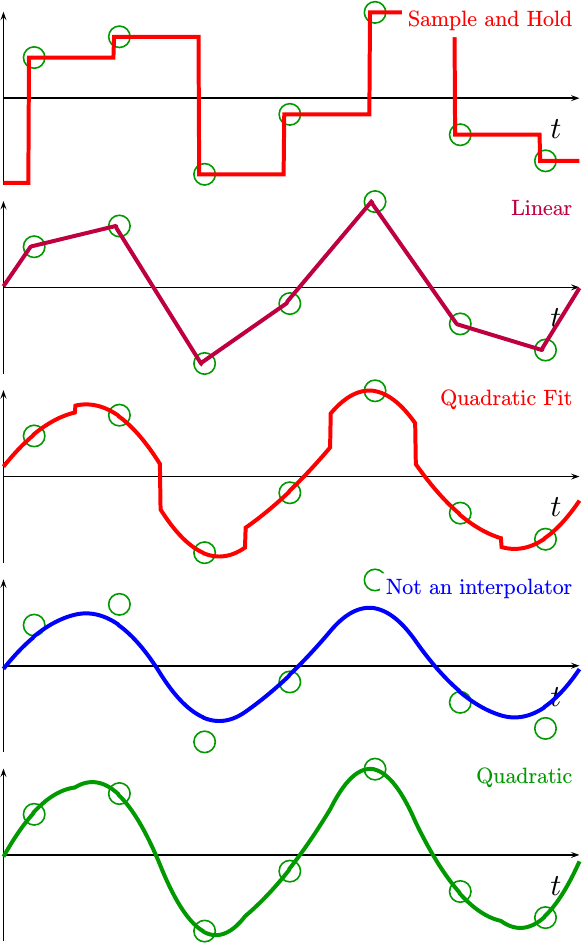
Quadratic fits are entirely inappropriate for DSP
Waveforms in nature have two characteristics that are difficult to handle in signal processing applications: natural waveforms are continuous and they are tend to last for a long time.
This is to be contrasted to the “signals” that Digital Signal Processing (DSP) algorithms act upon. DSP algorithms are applied to finite sections of (typically) longer waveforms that have been sampled at evenly spaced intervals.
This leads to a fundamental problem: if you want to work on a waveform as though it were continuous instead of sampled, then you need to figure out how to reconstruct what the signal should be between the sample points. Perhaps you need to resample that signal at some new rate whose ratio is far from simple when compared to the old rate. Perhaps you need to resample your signal at locations driven by a tracking loop, such as a digital receiver would need to do. Perhaps you just want to zoom in on a screen plot of your signal and linear interpolation leaves you with a signal that looks nothing like the original reality. Either way, if you want to recover what your signal does between samples, you’ll want to apply some form of interpolation.
In the past, we’ve looked at both a sample-and-hold “interpolator” and a linear interpolator as possible subsample interpolation methods. However, if linear interpolation isn’t good enough for your application, then the next best approach is some form of quadratic interpolation. Indeed, it’s not that hard to take three points and generate a quadratic that will pass through all three of them.
Stop. Now. Don’t do that. Really. Don’t.
In a moment I’ll show you why not. Then I’ll show you a better approach. Further, when implemented in logic, this better approach will still use only the same two hardware multiplies that a quadratic fit would’ve used.
Why interpolation
Interpolation is the term used to describe an algorithm that can be used to create (or estimate) data points between samples. This is often called upsampling in a Signal Processing context, with the difference between interpolating upsamplers and those that are not interpolating is that the output of an interpolator is guaranteed to go through the original sample points, whereas this is not necessarily the case of a more generic upsampler.
Today, we’ll be discussing interpolators that are also infinite upsamplers, such as those we discussed earlier when proving that all such interpolators could be modeled as convolutions of discrete-time signals with a continuous time filter. Such interpolators can form the basis of an asynchronous sample rate converter. For our purposes today, though, we will limit our discussion to interpolators which are simply the result of a piecewise polynomial upsamplers. We’ll even limit the discussion further to that subset of all piecewise polynomial upsamplers that is formed from quadratic polynomials.
I first learned the idea of polynomial upsampling from Harris, although it seems as though Farrow was the actual originator of the idea. Hence, you might recognize our ultimate solution as a Farrow filter, although it may not look like any Farrow filter you’ve seen before. Even better, it will have provably better asymptotic out of band performance than any Farrow filter or approach I’ve seen published to date.
The Problem with Quadratic Fitting
I started out this post by declaring that using a quadratic fit to the nearest three points were a horrible means of upsampling. Let’s take a moment before going further to see why this is the case. We’ll do this by first creating a fit to the nearest three points of a signal, and then examining what happens when you extend this fit beyond those three points into the points nearby.
As with any
interpolation
problem, we’ll start with a signal, x[n]. I’ll
use the square brackets, [], to emphasize that this is a
sampled signal
and hence only integer indices are allowed. From this
sampled signal,
our goal will be to create a new signal, y(t), with a
continuous
index, t–herein noted by the parentheses, ().
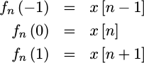
To create a quadratic fit, well pick three points from this signal,
x[n-1], x[n], and x[n+1], and then fit a quadratic function, f_n(t)
to these three points so that:
 |
Further, if we assume that our samples are spaced one unit apart, then
 |
The constant term of this quadratic
polynomial
is very simple to solve. If we examine t=n, then,
 |
The linear term is just a bit harder, but it can be obtained by subtracting
f_n(-1) from f_n(1),
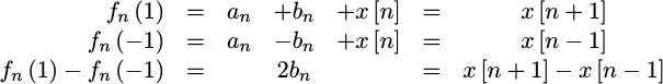 |
In other words,
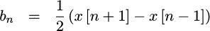 |
Getting the last coefficient is just a little bit more work, but follows from
adding the two end point values, f_n(1) and f_n(-1) together,
 |
This yields our quadratic coefficint,
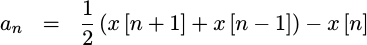 |
Therefore, we can fit any three sample values to the polynomial,
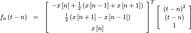 |
Fig 1 shows an example of one such fit.
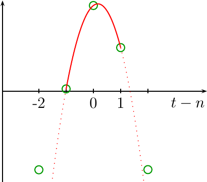 |
At first glance, this looks pretty good. We started with three data points, and now we’ve created a continuous line that smoothly interpolates between these three data points. What could the problem be?
The problem comes into play when you expand out from these three data points and examine the infinite set of samples that are the incoming data. In this case, the quadratic fit turns from a nice continuous interpolator, to discontinuous interpolator, where the discontinuity takes place halfway between any pair of samples.
 |
What happened?
What happened was that we chose to only use f_n between n-1/2 and
n+1/2. Once past n+1/2, we switched to a new
polynomial,
f_{n+1}. Since we did nothing to constrain our
polynomial
solution so that it was
continuous
between data sets, the result wasn’t
continuous.
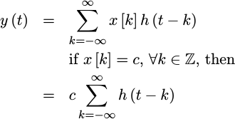
Before going further, let’s consider my previous statement that “Interpolation is just a special type of convolution.” Why? Because if you can understand this quadratic interpolator as just a convolution of your data with a continuous function,
 |
then we can plot the frequency response of this interpolator. Knowing that frequency response will allow us, further on, to compare this quadratic fit with other alternative quadratic interpolators.
To see how this fits into the form of a filter’s
impulse response, let’s
examine what happens when this
interpolator
is applied to an
impulse.
If we allow x[n] to be a
Kronecker delta function,
where x[n]=0 for all n save for x[0]=1, then the result of applying
this quadratic fit to this
sequence
will be the impulse
response
of this interpolator. Let’s do
that now.
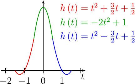
First, f_{-1}(t+1) will
sample
x[0]=1 in it’s n+1 term, yielding the
polynomial,
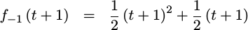 |
Likewise, f_{0}(t) will
sample
x[0]=1 in it’s n term, yielding,
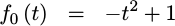 |
Next, the f_{1}(t) term will
sample
x[0]=1 in it’s n-1 term, giving us
our final piecewise
polynomial component,
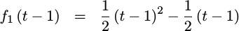 |
Put together, you can see this piecewise polynomial plotted out in Fig 3.
 |
See what happened? This impulse response isn’t continuous at all! This is the reason why our interpolated signal wasn’t continuous either.
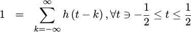
Further, it only takes some basic integral calculus to plot the frequency response of this function in Fig 4. (I’ll spare you the calculation–while basic, it isn’t pretty.)
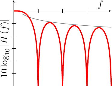 |
The gray line in Fig 4 is proportional to 1/f, showing how this
frequency response
only slowly converges towards zero as f goes to infinity. This is the
consequence of the discontinuities in the
impulse response
of this fit.
Now that you see the problem with using a simple quadratic fit as an interpolator, let’s see if we can do better.
A Better Interpolator
 |
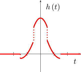
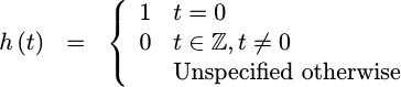
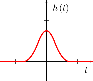
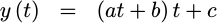
Now that we know what can go wrong with a piecewise polynomial interpolator, it’s time to return to where we left off in our prior post on this topic, and use the principles we developed there to develop a better interpolator. In that post, we showed that all interpolators that met a minimum set of problem related assumptions have the form of a piecewise polynomial, such as is shown in Fig 5.
Further, we pointed
out
that an h(t) function that is given by a
piecewise
polynomial,
such as the one shown in Fig 5, can be a
linear,
discrete shift invariant,
upsampler.
In Fig 5, you can see separate regions of an example filter, h(t), shown
in separate colors. Each colored region represents a separate quadratic
polynomial. Our goal will be
to try to use some criteria to create a useful set of
polynomials.
As a first step to building our own, let’s define our component piecewise polynomials as,
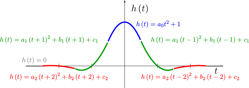 |
That is to say, we’re going to look for a
piecewise
polynomials
function, h(t), defined by the equations,
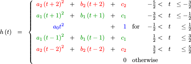 |
Why only five intervals? This is an arbitrary choice. There’s no hard and fast rule here. More intervals or a higher polynomial degree might produce a better filter, but one that will cost more logic to calculate. Such longer filters can be the topic for another discussion on another day. I do know that this setup will yield a nicely implementable solution ultimately requiring only two RTL multiplies.
Two multiplies you ask? What about all those arbitrary coefficients in h(t)?
Hang on, we’ll get there.
Why is there no b coefficient for the middle interval? Or, equivalently,
why are the *_1 and *_2 coefficients repeated? Because I have chosen a
symmetric
interpolation
filter, in the hopes of achieving a
linear phase
result. Further, I’ve started this derivation often enough without
pre-specifying these certain coefficients, and I end up specifying
them via equations anyway. By doing it this way, it just reduces the
number of coefficients we’ll need to solve for from the beginning.
To get to our result, all that remains is to determine the coefficients of the piecewise polynomials in our chosen filter. To do this, we’ll use some (rather ad-hoc) criteria to set up a system of linear equations to yield the as yet unknown coefficients.
- Interpolator
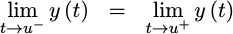
Our first criteria for h(t) is that the resulting waveform needs to
interpolate
the incoming waveform. In other words, whenever t is
an integer, the output value should equal the input. That is, if t=n
then y(n) = x[n].
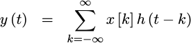
If we work this from the equation standpoint,
|
you can see that if t=n then y(n) is composed of a summation across
several h(t)
values, each with the index n-k. Further, when n=k we get the one
component we want, and all of the other components will just pull us off in
one direction or another. Hence, we need to insist that,
 |
 |
This means that every one of our
piecewise
polynomial component
functions, save the one in the center, will need to go through zero
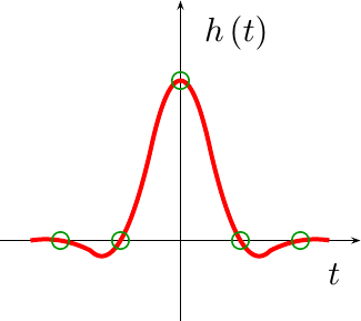
near the integer within it, as shown in Fig 6. The point in the center,
on the other hand, will need to pass through y=1.
It shouldn’t take too much work to see that our set of
piecewise
polynomial will
meet this criteria if we simply set c_1 and c_2 to be zero. Indeed,
this is the reason why it was constructed it based upon t-n terms in the
first place.
DSP Guru Meditation: It can be shown that if h(n) is a
Kronecker Delta function,
then it must also be true that,
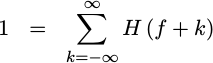 |
or, equivalently,
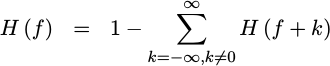 |
This, plus the fact that h(t) is real, forces the awkward reality
that H(1/2) must be 1/2 as well for all practical
low-pass
filters. Hence, this criteria alone forces the
passband and
stopband
cutoff frequencies of any
interpolator
to be f=1/2. This is a somewhat unfortunate limitation on the
performance that might be achieved using this approach.
This criteria is also a point of separation from Farrow’s work, since Farrow never insisted that the resamplers he developed went through the original sample points.
- Constant -> Constant:
x[n]=cimpliesy(t)=c
When I built my first Farrow interpolation filter from a quadratic piecewise polynomial, I was surprised to discover that a constant input to my filter was producing a non-constant output. Instead, there was a small but repeating quadratic component. How could this to happen?! How could I call this an interpolator, if the resulting interpolated waveform didn’t smoothly go through the given points?
So I then went back to my equations for h(t) and the coefficients of the
component polynomials,
and rebuilt them to insist that if x[n] is the constant c, then
y(t) should equal that same constant c as well.
Let’s do that here. With just a little manipulation, you’ll see that,
 |
Hence, we’ll want
 |
for all possible values of t between -1/2 and 1/2.
We can apply this criteria to our piecewise polynomial filter without too much hassle. I’ll spare you the gory details, although you should know that the result is a set of equations further constraining our polynomial coefficients.
If we continue solving for our eight coefficients, we’ll still need some more equations.
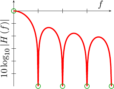 |
DSP Guru Meditation:
If you examine this property in
frequency,
it forces a unique and very desirable property upon the
interpolating
filter’s
frequency response.
In particular, the Fourier
transform of a constant
sampled
input has a component at X(e^{j0}) only, with X(e^{j2pi f})=c delta(f),
where delta(f) is the
Dirac delta function.
This would normally create aliasing components at frequencies X(e^{j2pi m})
for all integers m as well. However, we just insisted that for a constant
input, the Fourier
transform of the
continuous
output function was to have a component at zero only. Hence, we know that
X(e^{j2pi f})H(f) must be nonzero for f=0, and so we now know that
H(0)=1. We also know that H(m) must be zero for all integers m!=0,
H(m)=0–just like a sinc
function although other
functions can have this property as well.
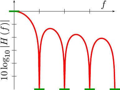
You can see this property shown in Fig 7 on the right.
- Linear -> Linear:
x[n] = nimpliesy(t)=t
Let’s follow that last criteria a bit further. Instead of just insisting
that every constant produce a constant signal output, we can also insist
that every linear input produce a linear output. Hence, if x[n]=n,
then y(t) should equal t.
As with our last criteria, we’ll apply our input, x[n]=n, and then
insist that the result contains no t^2 terms. (We already know it will
contain no constant terms.)
 |
This will give us another linear constraint on our coefficients.
DSP Guru Meditation:
If you examine this criteria in
frequency, it basically
forces the slope of H(m) to be zero for integers m. To be effective,
this criteria is dependent upon the constant criteria described above.
This constraint therefore not only increases the width of our pass band, but it also increases the depth of the nulls.
- Quadratic -> Quadratic:
x[n] = n^2impliesy(t)=t^2
For our fourth criteria, we’ll insist that if x[n]=n^2 then y(t) should
equal t^2. In many ways this is similar to the linear criteria above.
As with the linear criteria, this also provides us with another equation
to add to the system of equations we are building to solve for h(t).
DSP Guru Meditation: This criteria constrains the second derivative of
the frequency response
near both f=m for all integer frequencies m, thus also widening our
passband, as well as the width of the nulls in the
frequency response.
As a result, this criteria only intensifies our last constraint.
- Continuous:
As a final set of criteria, we’ll insist that our
piecewise
polynomial
impulse response be
continuous.
Hence, the h(t) function must be
continuous
at its seams: t=-5/2, t=-3/2, t=-1/2, t=1/2, t=3/2, and t=5/2.
However, since we constrained our
piecewise
polynomial to be
symmetric
in time, we really only need to deal with half of those t values.
Because any linear combination of
continuous functions
is also
continuous,
y(t) will be
continuous
any time h(t) is
continuous.
There’s an even more important consequence of this ad-hoc criteria: any
continuous function
will have a frequency
response.
with an asymptotic decay proportional to 1/f^2 or better. This function
is no different. Hence, when you put all of our constraints together, we’ve
now constrained the zero frequency, f=0, and the first and second
derivatives of all integer frequencies. By now insisting on a
continuous
impulse response,
we’ve also constrained the asymptotic frequency
response of this
interpolating
filter as well.
In other words, we’ve just created an interpolating function with a very nice low-pass frequency response–it just doesn’t have a very narrow transition band.
DSP Guru Meditation: I will contend, based more upon frustration then
proof, that it is actually impossible to create a finite quadratic
interpolating
polynomial via this method that
will be continuous in
its first derivative. Before you jump to disprove me, remember my definition
of an
interpolating
polynomial, which requires that it
equal zero at all integer locations but zero. Were we able to create such a
function, it would have an out of band asymptotic decay rate of 1/f^3–but
we’ll leave the discussion of such functions for a later discussion of either
higher order interpolators,
or quadratic splines.
As an aside, it is possible to formulate the splines problem in this fashion. Doing so produces a solution that no longer requires solving for the piecewise polynomial to be coefficients at every step, while yielding a cleaner and (slightly) wider passband.
If you put all of the resulting equations together, for the constraints outlined above, you will get an over-determined system. This over determined system will include several redundant equations which can be easily removed. Once the redundant equations are removed, you will then get the system of linear equations below.
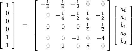 |
In spite of starting with an over determined system in this process, we got lucky: the system above has a unique solution given by,
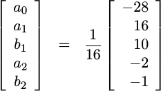 |
Wow, that was a lot of work to just get a bunch of numbers. So what, right? What’s the use of these five values?
The value of this solution is seen in the impulse response and frequency response shown in Fig 9.
 |
As we required, the
passband and
is “flat” near f=0, and the nulls are deep.
Unlike both the nearest neighbor
interpolator
and the quadratic fit we
discussed above, the asymptotic fall off of this filter is proportional to
1/f^2. Further, unlike the linear interpolator we built
earlier
which also has an asymptotic fall off of 1/f^2, this
asymptotic fall off has a smaller proportionality coefficient of 1/f^2.
For comparison, consider Fix 7 above showing the
frequency response
of the linear
interpolator.
In other words, this quadratic interpolator forms a nice piecewise polynomial interpolation filter.
Even better, with some careful coding (below) we can implement the coefficient multiplication with only adds and subtracts. This will mean that we can evaluate this quadratic in Verilog using only two hardware multiplies–minimizing a precious resource found within any digital logic component.
Sadly, the development above is only an ad-hoc formulation. While it may be possible to truly generate optimal interpolators via this method, I have not yet pursued such a study in depth.
Three Interpolators and only Two Multiplies
In the next section, we’ll start discussing how to build the Verilog code necessary to implement this interpolator. Indeed, well even do one better than that: we’ll show the Verilog code necessary to implement three separate quadratic interpolators–all with only two multiplies.
- The first interpolator will be the one that results from the quadratic fit approach I was so critical of above. We’ll use this performance for reference below. This interpolator is given by the equations we developed above:
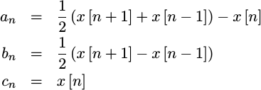 |
As we discussed above, we can expect this interpolator to produce a discontinuous output waveform.
- The second upsampling
function may have the best stopband
performance among all quadratic
upsamplers, however it’s not a true
interpolator
since it doesn’t necessarily go through the original signal
sample
points. We’ll call this the
non-interpolator
for lack of a better term. This
non-interpolator
is a very valuable
upsampling
function for the simple reason that its
frequency response
tail falls off faster (
1/f^3) than any other quadratic. Indeed, it is so valuable, that we may come back and use it to beat the performance of a CORDIC–but that will have to be the topic of a future article (it will still require two multiples, something the CORDIC doesn’t need).
 |
 |
This non-interpolator will not suffer from the discontinuities we discussed above. Further, if you are up to a calculus challenge, this function can be derived by convolving a rectangle function with itself three separate times, hence its impulse response is shown in Fig 11.
One unique feature of this upsampler is its properties when doing peak finding. Indeed, peaks found following this fit tend to be more accurately located than when using the interpolator that is the topic of today’s development–but this again is a topic for another day.
Since the non-interpolator’s impulse response response is created by convolving a rectangle function with itself three separate times, its frequency response will be given by the frequency response of a rectangle function cubed, or in other words by a sinc function cubed.
Further, if you compare the coefficients of this
the non-interpolator’s
impulse response
with those of the quadratic fit (above), you’ll see that all but the
constant coefficients, c_n, are identical.
In our code
below, the parameter OPT_IMPROVED_FIT will control whether or not this
non-interpolating
upsampler
is generated or not. If set, the traditional quadratic fit will be bypassed
for this alternative implementation.
DSP Guru Meditation: My statement above that the
frequency response
tail of this filter asymptotically decays faster than any other quadratic
isn’t quite true. Quadratics filters composed of a linear combinations of
this filter function will also fall off at the 1/f^3 rate … but we’ll
leave the further discussion of this approach to a future discussion of
quadratic (and/or cubic)
splines, since that’s
where it is most relevant.
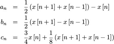
- The third function we’ll implement is defined by the coefficient equations we just developed in the last section above.
 |
This is the one we expect to see good results from–it is
continuous,
and passes constants, lines, and quadratics without distortion. Not
only that, the
interpolator
generated by this function is guaranteed to go through the initial
x[n]
sample
points given to it.
The parameter OPT_INTERPOLATOR in
our code below
will control whether or not this
implementation is used. If set, OPT_INTERPOLATOR will override the
OPT_IMPROVED_FIT option parameter above, yielding an implementation of
this quadratic
interpolator.
We’ll use some careful coding techniques in the next section in order to avoid using hardware multiplication elements when multiplying the quadratic coefficients generated by the incoming data by these factors, 28, 16, 10, 3/4, etc. The resulting algorithm will use only shifts and adds–up until the final quadratic evaluation. We will need to be careful to make certain that we track the decimal point during this process though.
When it comes to evaluating the polynomial itself, if you’ve never implemented one numerically, then you should know that there is a right and a wrong way to apply the multiply–a “trick” if you will. In particular, you don’t want to calculate your result by a straight forward evaluation,
 |
This straight forward approach suffers from two problems. The first problem is that it costs three multiplies. (Ouch!) The second problem is that this method is susceptible to the loss of precision as the intermediate values are truncated prior to their final addition.
Instead, we’ll calculate this polynomial’s value based upon a different formulation:
 |
This will solve both of these problems, yielding a nice solution suitable for RTL implementation.
Fixed Point
Let’s pause for one more section before diving into the code below, to discuss how we are going to handle the evaluation of the piecewise polynomial function coefficients.
Our first step will be to replace the polynomial, coefficients with elements of a sample based shift register.
always @(posedge i_clk)
if (i_ce)
	{ x[3], x[2], x[1], x[0] } <= { x[2], x[1], x[0], in };
This will eliminate the dependence of the algorithm on the integer n.
We’ll use the input data as the first element in this registers,
and use x[0] to refer to the prior input, x[1] to refer to the value
before that, etc. Hence, we’ll map the following values:
| Old name | New Name |
|---|---|
| x[n+2] | in |
| x[n+1] | x[0] |
| x[n+0] | x[1] |
| x[n-1] | x[2] |
| x[n-2] | x[3] |
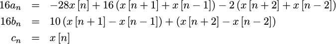
This allows us to re-express the above filter coefficient equations as,
   16 av = 4(x[1]-8x[1])+16(x[0]+x[2])-2(in+x[3])
   16 bv = 2[(x[0]-x[2])+4(x[0]-x[2])]+(in-x[3])
   cv = x[1]
You may also notice that all of the multiplies necessary to calculate
the coefficients, a_n, b_n, and c_n,
have now been replaced with adds and shifts. Instead of multiplying by -28
for example, we can subtract 8x[1] from x[1] and then shift the result left by two bits. In a similar fashion, we can multiply x[0]-x[2] by five
by adding x[0]-x[2] to 4(x[0]-x[2]). The final multiplication by
two, or rather left shift by one, just completes the desired multiply by ten.
Even this is too hard, though, since it will take us a couple of clocks to calculate these values. Hence we’ll go about calculating our coefficients in three steps each in a different clock cycle.
We’ll start, therefore, by splitting this process into three sets of operations. Eventually these will take place on separate clock cycles, but for now we can draw them out as though they all happened at once.
   pmidv = 8x[1] - x[1]; // = 7x[1]
   psumn =  x[0] + x[2];
   difn  =  x[0] - x[2];
   //
   diffn = difn + 4difn;	// = 5 * (x[0] - x[2])
   sumw  =   in  + x[3];
   diffw =   in  - x[3];
   midvpsumn = 4(psumn) - (pmidv); // = 4(x[0]+x[2])-7x[1]
   //
   16 av = 4(midvpsumn)-2(sumw)
   16 bv = 2(diffn)+(diffw)
   cv = x[1]
This can then be rewritten into pseudo-RTL logic over the space of three clock
cycles. Our notation for the shift register components from before, in
through x[3], will be valid on the second clock cycle. Hence, for the
first clock we’ll be referencing in through x[2] instead of x[0]
through x[3].
always @(posedge i_clk)
if (i_ce)
begin
   // First clock, pre-data
   pmidv <= 8x[0] - x[0]; // Was 8x[1] - x[1]
   psumn <=   in + x[1];  // Was x[0] + x[2]
   difn  <=   in - x[1];  // Was x[0] - x[2]
This takes care of some of the inner operations from our equations above. The next step handles some more of the “multiplies”.
   // Second clock
   diffn <= difn + 4difn;	// = 5 * (x[0] - x[2])
   sumw  <=   in  + x[3];
   diffw <=   in  - x[3];
   midvpsumn <= 4(psumn) - (pmidv); // = 4(x[0]+x[2])-7x[1]
In the final clock cycle we’ll calculate the actual coefficients. Because
FPGA
math is primarily fixed point, we’ll leave the 16 on the left–indicating
that we never divided by the necessary 16. We’ll need to drop the extra four
bits later, but for now we’ll leave them in
place as long as possible to avoid loss of precision.
   // Third clock, data delayed by one
   av <= 4(midvpsumn)-2(sumw); // * 2^4
   bv <= 2(diffn)+(diffw); // * 2^4
   cv <= x[2];
end
This gives us the coefficients of our piecewise polynomial for a given set of five input samples.
We still need to calculate the value of t that needs to be used when
evaluating this polynomial.
This logic will follow directly from the linear interpolator
development,
and is even copied from that development.
The only big difference between this and the linear
interpolator
development is that, unlike the
linear interpolator,
this piecewise quadratic
polynomial
interpolates
from around the
sample points
(|t|<1/2), rather than between
sample points,
(0<t<1).
Perhaps this would make more sense with a figure. Fig 12 therefore shows in color how the quadratic upsampler will interpolate from around the sample points on the left, rather than between the sample points as shown on the right.
 |
I’m not really sure why this is so, I just know that I haven’t managed to build a symmetric quadratic polynomial between sample points (right side of Fig. 12 above) that ended up being very useful. To handle this difference, we’ll keep track of the last coefficients.
always @(posedge i_clk)
if (i_ce)
begin
	avold <= av;
	bvold <= bv;
	cvold <= cv;
end
Then, if our local t value is less then zero (MSB is set), we’ll
use the newer coefficients, av-cv, otherwise we’ll use the
older, delayed by one avold-cvold coefficients.
We’d also like to add a half to t at this point, so that it ranges between
0 and 1 instead of from -0.5 to 0.5. It turns out that’s not needed.
t naturally fits into place without change–all that’s required is to
re-interpret the signed t value as an unsigned value and the conversion
is done.
That gives us our three coefficients, r_av, r_bv, and r_cv,
together with our time offset, r_offset.
Finally, as we go through the rest of the algorithm, we’ll use the prefixes
r_, qp_, ls_, and lp_ to indicate which stage of the quadratic
algorithm we are in.
-
The
r_prefix will hold the first copies of our variables in the “new” sample rate domain. This will include not only the quadratic coefficients,r_av,r_bv, andr_cv, but also the value oftassociated with these coefficients, held inr_offset. Finally,r_cewill be true on any clock where these values are valid. -
The
qp_prefix will hold our variables immediately after taking the quadratic product,a*tor in terms of our registers,r_av * r_offset. -
The
ls_prefix will refer to the variables associated with the linear sum, the result of addinga*t+bor equivalently the output of the quadratic product plusr_bv. -
The
lp_prefix will denote values associated with multiplying this last product and linear sum by ourtvalue one more time to get(at+b)*t. As a result, when we add the constant to the result of this last multiply, we’ll have our final value which we shall callr_done.
The algorithm below doesn’t do any rounding until the final step. Instead, it accumulates a lot of extra bits along the way, so that there’s not that much precision lost along the way.
The Code
We’ve now made it far enough in our description that we can now walk through the algorithm. Feel free to skip this section if you would like and go directly to the performance section below, and then return to this once you’ve become convinced that you really are interested in the algorithmic details. You can also just examine (or implement) the code, yourself to see what your thoughts are of it.
The algorithm starts by defining some interface parameters.
	parameter	INW   = 25,	// Input width
			OWID  = INW,	// Output width
			MP    = 25,	// Multiply precision
			CTRBITS = 32;	// Bits in our counter
These are the input width, the output width, and the number of bits of our
time counter to use in the multiply. The fourth value, CTRBITS, controls
the total number of bits in the time counter. In other words, how accurate
the fractional
upsampling
ratio should be. As with the linear
interpolator
development, this counter will step, on each input
sample,
by a step size given by the input i_step,
i_step = 2^(CTRBITS) (int)(old_sample_rate / new_sample_rate);The number of bits in CTRBITS will just control the accuracy and precision
of the
resampling
function.
The next two parameters, OPT_INTERPOLATOR and OPT_IMPROVE_FIT, we
discussed earlier. These control which quadratic
resampler
to implement among three defined in the code. OPT_INTERPOLATOR=1 will
cause us to use the new
interpolator.
On the other hand, if OPT_INTERPOLATOR=0 but
OPT_IMPROVED_FIT=1, then we’ll use the
non-interpolator
output. Finally, if both are zero the algorithm will calculate the
quadratic fit I’ve been so critical of.
	parameter  [0:0]	OPT_IMPROVED_FIT = 1'b1;
	parameter  [0:0]	OPT_INTERPOLATOR = 1'b1;
The last parameter, GAIN_OFFSET, controls how far we shift the final result
to the right. Ideally, this would be 4 if OPT_INTERPOLATOR would be set in
order to divide by the factor of sixteen shown above. Sadly, we can’t do that.
In particular, a set of constant maximum negative values surrounding a maximum
positive value, or vice versa, will yield filter results outside of that
incoming range. Hence, to avoid overflow, we’ll only shift by three bits
(divide by eight), or two for the quadratic fit approaches.
parameter GAIN_OFFSET = (OPT_INTERPOLATOR)? 3:2;The next step is to calculate the bit widths of various portions of this algorithm. These are held in local parameters, since they are calculated from the main parameters above. The first are the bit widths of the coefficients,
			// Bit-Width's of the quadratic, linear, and constant
			// coefficients
	localparam	AW = (OPT_INTERPOLATOR)?INW+6:INW+2,
			BW = (OPT_INTERPOLATOR)?INW+6:INW+1,
			CW = (OPT_INTERPOLATOR)?INW  :((OPT_IMPROVED_FIT)?(INW+3):INW),
followed by the number of bits we’ll have after the decimal place following each computation,
			ADEC=(OPT_INTERPOLATOR)? 4:1,
			BDEC=(OPT_INTERPOLATOR)? 4:1,
			CDEC=(OPT_INTERPOLATOR)? 0:((OPT_IMPROVED_FIT)? 3:0);
Remember, any time you want to multiply integers and fractions such as A.B
times X.Y (not the decimal place), you’ll need to first move the decimal
place to the far right so as to get 2^N(AB.) and 2^M(XY.). Then, when
you multiply these numbers, you can shift them back to get the result you
were looking for back to where it belongs:
A.B * X.Y = (AB. * XY.)*2^(-N-M)Of course, in practice this just means that we’ll track this resulting decimal point, as you’ll see through the code.
The final local parameter is the width of the internal calculations. This is the number of bits that we will keep following each multiply.
	localparam	BMW = ((AW-ADEC>BW-BDEC) ? (AW-ADEC+BDEC) : BW);
	localparam	CMW = ((BMW+1-BDEC>CW-CDEC) ? (BMW+1-BDEC+CDEC) : CW);
With these preliminaries aside, we can finally dig in to the implementation of our quadratic interpolator, beginning with how we generate the polynomial coefficients themselves. Since this will change depending upon our choice of quadratic, we’ll use a generate block to select from among several logic sets.
	generate if (OPT_INTERPOLATOR)
	begin
As our first step, we’ll calculate the shift register of data inputs and a short history that we discussed above in the last section.
		always @(posedge i_clk)
		if (i_ce)
			{ mem[3], mem[2], mem[1], mem[0] }
				<= { mem[2], mem[1], mem[0], i_data };
Let’s take a moment here to discuss i_ce. This is the “global CE” signal
from our previous discussion on pipeline
strategies.
As you may recall from that
discussion,
the “global CE strategy” is very appropriate for
signal processing
applications. Further, you’ll want to remember the rules associated with the
“global CE” signal: Nothing changes except on the clock that i_ce is true.
Since this is a
resampling
module, though, we’ll have to extend this rule. Nothing on the incoming
sample
rate side changes unless i_ce is true.
We’ll use another CE signal, r_ce for the output
sample
side in a moment.
The next several calculations also follow directly from the last section as well. The only difference here is that this time we are applying the necessary shifts to accomplish the needed “multiplies” from before.
		always @(posedge i_clk)
		if (i_ce)
		begin
			pmidv <= { mem[0], 3'b000 }
					- { {(3){mem[0][INW-1]}},mem[0]};// x7
			psumn <= { i_data[(INW-1)], i_data }
					+ { mem[1][(INW-1)], mem[1] };
			pdifn <= { i_data[(INW-1)], i_data }
					- { mem[1][(INW-1)], mem[1] };
			//
			sumw <= { mem[3][(INW-1)], mem[3] }
					+ { i_data[(INW-1)], i_data };
			// sumn <= psumn;
			diffn<= { pdifn[INW], pdifn, 2'b00 }
					+ {{(3){pdifn[INW]}},pdifn };// x5
			diffw<= { i_data[(INW-1)], i_data }
					- { mem[3][(INW-1)], mem[3] };
			// midv <= pmidv;
			midvpsumn <= -{ pmidv[(INW+2)],pmidv }
					+ { psumn[INW], psumn, 2'h0 };//-x7+ x4
		end
That’s the first two clocks. Then, on the third clock, we use these
intermediate expressions to generate the actual quadratic coefficients.
Remember, though, the mem[x] values by this clock have shifted forward by
one extra
sample.
As a result, cv is set to mem[2] instead of mem[1].
Likewise, the av and bv values here have been multiplied by sixteen
compared to the coefficients we want. This factor of sixteen will ultimately,
and only partially, be corrected with the GAIN_OFFSET when we are done.
		initial	av = 0;
		initial	bv = 0;
		always @(posedge i_clk)
		if (i_ce)
		begin
			// av = x28 + x16 + x2
			// av = - { midv, 2'b00 } + { sumn, 4'h0 } - { sumw, 1'b0 };
			av <= { midvpsumn, 2'b00 }
					- { {(4){sumw[INW]}}, sumw, 1'b0 };
			bv <= { diffn[INW+3],diffn, 1'b0 }
				- { {(5){diffw[INW]}}, diffw };
			cv <= mem[2];
		end

	end else begin
The next two sections in the code calculate the coefficients of the quadratic fit and our non-interpolating quadratic. We’ll skip these here for simplicity, so that we can focus on today’s quadratic interpolator, however we’ll show the results of these upsampling filters further down.
At this point, then, we have our three quadratic coefficients, av, bv,
and cv–regardless of which algorithm generated them.
We discussed in the last section the need for keeping the coefficients from the last interval around, so we’ll copy them here.
	always @(posedge i_clk)
	if (i_ce)
	begin
		avold <= av;
		bvold <= bv;
		cvold <= cv;
	end
We’ll resample our data two clocks following any new incoming data, so let’s capture that new value here.
	always @(posedge i_clk)
		pre_ce <= i_ce;
That brings us to calculating when to take our next sample. This code should be familiar, as it was lifted from our discussion on linear interpolators.
First, we calculate the when of the next
sample
point. Our t value is given by this counter. When the counter overflows,
the next outgoing
sample
will require a new incoming
sample
so we’ll then stop moving forward and wait for that next
sample
	// ...
	initial	r_ovfl  = 1'b1;
	always @(posedge i_clk)
		if (i_ce)
			{ r_ovfl, r_counter } <= r_counter + i_step;
		else if (!r_ovfl)
			{ r_ovfl, r_counter } <= r_counter + i_step;
In the end, the sample indicator is a combination of either following a new sample value, or any other sample up until the counter overflows. In this fashion, we’ll upsample the incoming data.
	// ...
	initial	r_ce = 1'b0;
	always @(posedge i_clk)
		r_ce <= ((pre_ce)||(!r_ovfl));
Please feel free to refer back to the linear interpolator series if you find this logic difficult to understand.
Two steps are left before evaluating the quadratic
polynomial: calculating t,
and switching our coefficients so that the quadratic function we create
surrounds our incoming data point. This accomplishes the transformation
illustrated in Fig 12 above.
	always @(posedge i_clk)
	if (r_ce)
		pre_offset <= r_counter[(CTRBITS-1):(CTRBITS-MP)];

	// ...
	always @(posedge i_clk)
	if (r_ce)
	begin
		r_offset <= { pre_offset[MP-1], pre_offset[(MP-2):0] };
		if (pre_offset[(MP-1)])
		begin
			r_av <= av;
			r_bv <= bv;
			r_cv <= cv;
		end else begin
			r_av <= avold;
			r_bv <= bvold;
			r_cv <= cvold;
		end
	end
At this point we now have our quadratic coefficients, r_av, r_bv, and
r_cv, together with our time offset, r_offset. These are the coefficients
of the quadratic we wish to evaluate. Indeed, at this point all of the
difficult stuff is done. All that remains is to handle the quadratic
evaluation itself.
The first step is to multiply a by t. To keep everything else aligned,
we’ll forward all of our other coefficients to the next clock.
	always @(posedge i_clk)
	if (r_ce)
	begin
		qp_quad  <= r_av * r_offset;	// * 2^(-MP-ADEC)
		qp_bv    <= r_bv;		// * 2^(-BDEC)
		qp_cv    <= r_cv;		// * 2^(-CDEC)
		qp_offset<= r_offset;		// * 2^(-MP)
	end
Many FPGA’s have dedicated multiply accumulate capability in their
DSP
hardware. Such a capability would allow
us to calculate r_av * r_offset + r_bv–with an appropriate bit select
along the way. For right or wrong, this has never been my coding practice.
Perhaps I just want more control of the operation. Either way, I will often
split these two calculations into two separate clocks. That’s why we aren’t
adding the bv coefficient to this multiplication result in this clock.
Before the next step, let’s consider what we have. We have three numbers,
with decimal points in varying locations. r_av for example has ADEC
bits following the decimal point, and we just multiplied it by a value, t,
all of whose bits were to the right of the decimal point. Hence, we now
have (MP+ADEC) bits following our decimal point in a number that is
AW bits wide. Let’s keep track of this decimal point as well as the
decimal point for qb_bv in our notes.
	// qp_quad (AW-ADEC).(MP+ADEC)
	// qb_bv   (BW-BDEC).(BDEC)
We are now going to want to add the results of this multiply to our b
coefficient in our next step. To do this though, we’re going to first
need to normalize
both values so that they have the same number of decimal points.
In spite of the ugly looking code below, we’re just dropping the extra
bits off the bottom.
	// lw_quad (BW-BDEC).(BDEC)
	assign	lw_quad = { {(BMW-(AW+MP-(MP+ADEC-BDEC))){qp_quad[(AW+MP-1)]}},
				qp_quad[(AW+MP-1):(MP+ADEC-BDEC)] };
Hence, we just shifted qp_quad down by (MP+ADEC-BDEC) binary decimal points,
so that it now has BDEC bits following the decimal instead of MP+ADEC.
The result, lw_quad, now has the same number of decimal places as
qp_bv, so we can now add these two numbers together. As before, we’ll
forward the constants we haven’t yet used to the next clock cycle.
	always @(posedge i_clk)
	if (r_ce)
	begin
		ls_bv    <= { {(BMW+1-BW){qp_bv[BW-1]}}, qp_bv }
				+ { lw_quad[BMW-1], lw_quad };
		ls_cv    <= qp_cv;
		ls_offset<= qp_offset;
	end
As a next step, we’ll calculate (a*t+b)*t and place the result into lp_bv.
	always @(posedge i_clk)
	if (r_ce)
	begin
		lp_bv    <= ls_bv * ls_offset;	// * 2^(-MP-BDEC)
		lp_cv    <= ls_cv;		// * 2^(-   CDEC)
	end
As before, we keep track of our decimal points at this step.
	// lp_bv (BMW+1-BDEC).(BDEC+MP)
	// lp_cv    (CW-CDEC).(CDEC)
This helps us to know how much to shift lp_bv by in order to align it with
lp_cv so that the two can be added in the next step.
	wire	signed	[(CMW-1):0]	wp_bv;
	assign	wp_bv = { lp_bv[(BMW+MP):(MP+BDEC-CDEC)] };
This brings us to the last part of calculating the quadratic, adding the constant to the final result.
	always @(posedge i_clk)
	if (r_ce)
		r_done <= { wp_bv[CMW-1], wp_bv }
				 + {{(CMW+1-CW){lp_cv[CW-1]}}, lp_cv};
And we’re done!
Okay, not quite. We still need to drop a bunch of bits. As we discussed earlier, there’s a right and a wrong way to do drop bits in a DSP algorithm. Hence, we’ll round towards the nearest even integer here and then throw the rest of the bits away.
	generate if (CMW+1-GAIN_OFFSET > OWID)
	begin : GEN_ROUNDING
		reg	[CMW-GAIN_OFFSET:0]	rounded;

		initial rounded = 0;
		always @(posedge i_clk)
		if (r_ce)
			rounded <= r_done[(CMW-GAIN_OFFSET):0]
				+ { {(OWID){1'b0}},
					r_done[CMW-GAIN_OFFSET-OWID],
				{(CMW-OWID-GAIN_OFFSET-1)
					{!r_done[CMW-GAIN_OFFSET-OWID]}} };

		assign	o_data = rounded[(CMW-GAIN_OFFSET)
					:(CMW+1-GAIN_OFFSET-OWID)];
The code contains two other non-rounding choices, which we shall skip here in our discussion.
The final step is to note when this output is valid. This involves forwarding our new global CE pipeline control signal to the output.
	// ...
	end endgenerate

	assign	o_ce = r_ce;

	// ...
endmodule
At this, we are now done and our code is complete. But does it work? Let’s see in the next section.
The Proof
I’ve always counseled individuals not to use a tool they aren’t familiar with. Every tool in the shed has its purpose, its capabilities, and its limitations. This interpolator is no different from any other tool in that sense. To see how well, or poorly, this quadratic interpolator works, let’s test it. In particular, we can sweep a sine wave through the input and see what happens. Further, let’s compare this interpolator with four different interpolation methods:
-
Our first method will be the simple sample and hold circuit we presented earlier. Since the code within this module doesn’t really handle upsampling, we’ll use the global CE from the other interpolators to know when to capture this output.
-
The second method will be a straight-forward linear interpolator.
-
Our third choice will be the quadratic fit we developed above, allowing you to see just how good, or poor, this interpolator is in practice.
-
We’ll then use the nice quadratic upsampler from above, the one that we chose to call the non-interpolator.
-
The final test algorithm is today’s quadratic interpolator algorithm.
While I won’t walk you through the test code (today), I will post it with the rest of the interpolator’s code in my interpolation repository. If you are interested in this test code, check out the bench subdirectories. There you will find a master Verilog module that instantiates examples of all of the filters below, as well as a Verilator based C++ program that will exercise these filters and write the outputs to a data file. Finally, there’s a Octave script that can be used to plot these results.
Sadly, the resulting data is too voluminous to plot in its entirety here, so I’ll just pick some useful and revealing sections of this data for discussion.
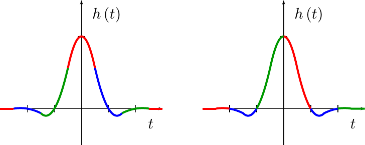
For four first example, let’s compare how these interpolation functions perform for a low frequency sine wave.
 |
By visual inspection alone, most of the quadratic interpolators did pretty well. Even the linear interpolator seems to be tracking the sine wave. quite nicely.
If you look even closer, though, you may notice some minor discontinuities in the quadratic fit, or locations where the quadratic non-interpolator doesn’t go through the given sample points. These effects are minimal at this low frequency, but they are present.
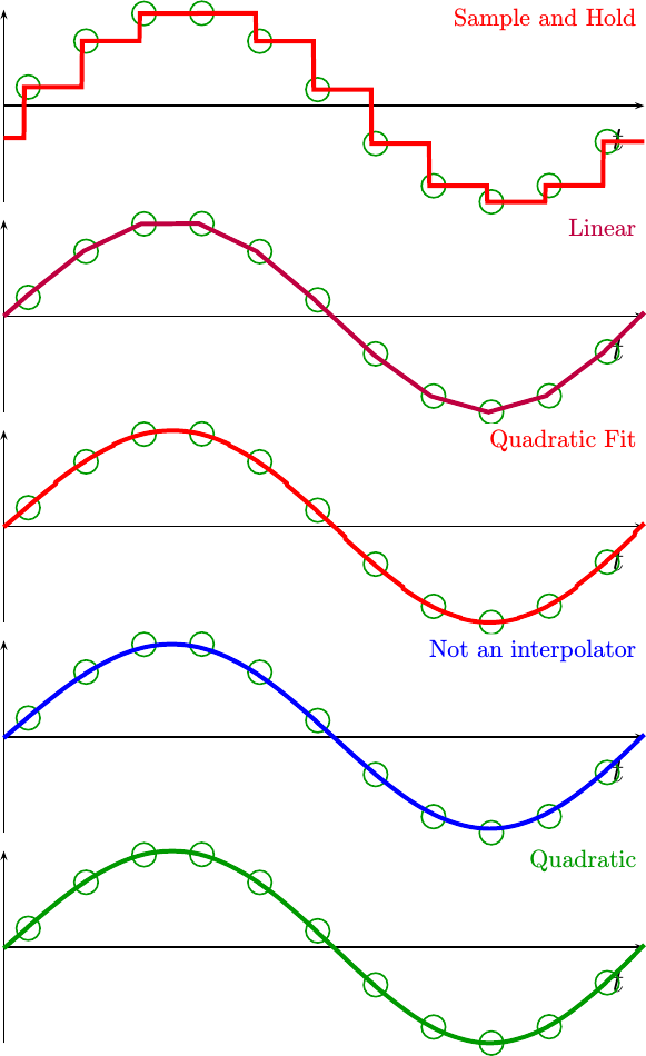
So, let’s increase the frequency.
Fig 14 below shows the same
sine wave,
but this time with a frequency between 0.25 and 0.3 cycles per sample.
 |
Here the differences become very stark. The quadratic fit’s discontinuities are much larger, and the non-interpolator is clearly missing the input sample points.
If you look closer, you may even see some kinks in the quadratic interpolator we just built. These are a result of the fact that, although this interpolator is continuous, it is not continuous in its first derivative. Achieving that result will take more work–something we’ll leave for another day. Even still, though, this is probably good enough for most purposes at this frequency.
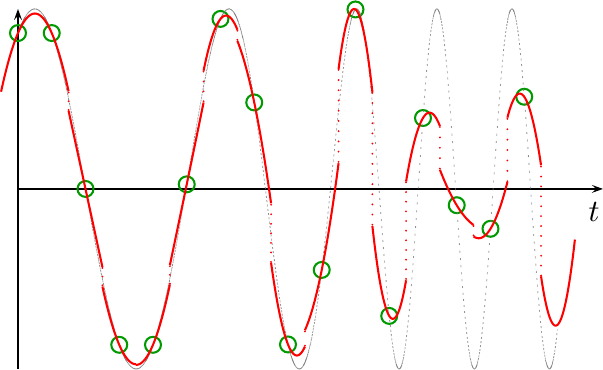
What about a higher frequency? Why not push both of these interpolators until they completely break down near the Nyquist frequency?
That’s the purpose of the next figure, Fig 15. In this figure, the incoming sine wave is sampled right near the Nyquist cutoff frequency of two samples per cycle.
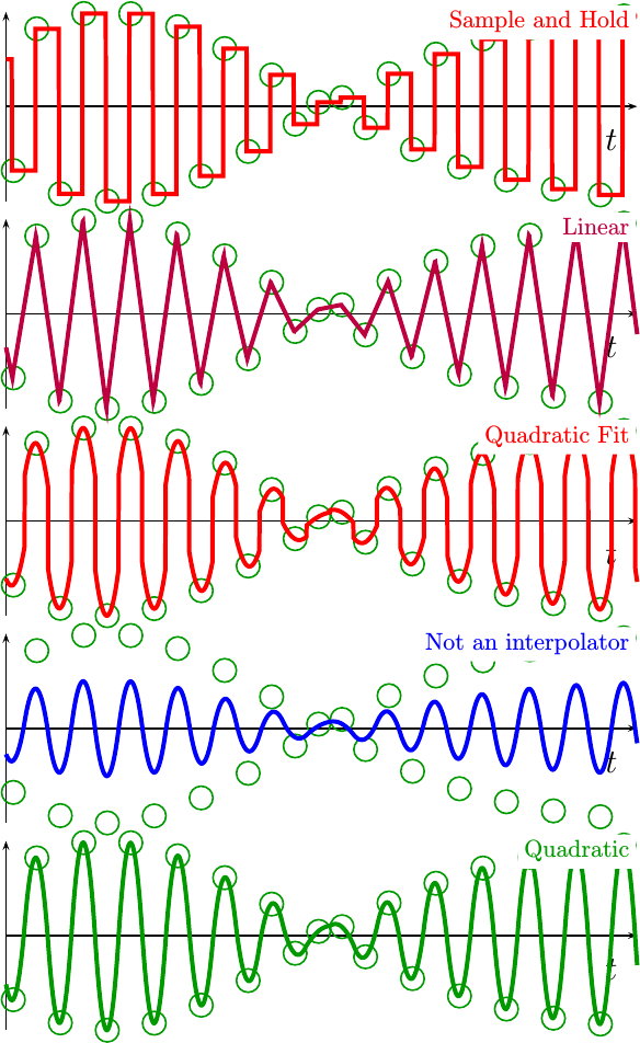 |
Judging from the images above, it looks like the interpolators are tracking the outline of a sine wave multiplied by some kind of envelope. The incoming signal, however, had no envelope function constraining it. Indeed, the incoming signal was nothing but a straight sine wave. Instead, this apparent “envelope” is the result of undersampling a high frequency sine wave.
Which interpolator is better in this environment? I might argue that none of them work well this close to the Nyquist frequency, and that instead this final example frequency is really beyond their capability. This isn’t to say that better interpolators do not exist, or that they cannot be developed. Rather, it is simply a statement of the reality that any interpolator will break down as it approaches the Nyquist frequency.
Conclusion
For just the cost of a couple multiplies, several additions and bit selects, and quite a few flip-flops, we’ve managed to implement a better interpolator. This interpolator is better than a sample and hold, better than a linear interpolator, and even better than the straight forward quadratic fit we started with. Further, unlike the more traditional Farrow filter development, the output of the resampler created by this interpolator is actually constrained to go through the input samples.
Does this mean that this is the best approach to interpolation? By no means. While this solution has some nice properties associated with it, it has no optimality properties. In that sense, it’s just another ad-hoc development in a similar vein to Farrow’s.
As with everything, though, you get want you pay for. Better interpolators of this variety exist, but they do cost more. For example, there’s another filter like this one documented in my interpolation tutorial, although the coefficient multiplies are too difficult to do with just adds and subtracts. Indeed, they require a divide by 80! Another approach is to use spline interpolation. You may remember my earlier suggestion that spline interpolation could be done without calculating a new matrix solution for every data point.
This, though, will need to be a discussion for another day.
And he spake also a parable unto them; No man putteth a piece of a new garment upon an old; if otherwise, then both the new maketh a rent, and the piece that was taken out of the new agreeth not with the old. (Luke 5:36)