
Implementing the Moving Average (Boxcar) filter
When we first examined filtering, we looked at the two simplest digital filters I knew of: a filter that averages adjacent values, and a filter that recursively averages multiple numbers together. These two simple filters required only a few FPGA resources, and so they were easy to implement. Sadly, they weren’t very configurable and so their filtering capability was quite limited.
We then came back to the topic and discussed how to create a generic Finite Impulse Response (FIR) filter. Such a generic FIR filter is very configurable. Using the approach I presented, you can describe any FIR digital filter in logic. We then came back to the topic a bit later, and discussed how to create a filter that required fewer flip-flops, while still maintaining the complete configurability of any generic FIR filter.
The problem with both of these generic approaches is their cost. As with most digital filters, this cost is often measured in the number of multiplies (i.e. the number of taps). While the number of logic blocks and flip-flops is also of interest, even this logic scales with the number of filter taps required.
As an example of this problem, suppose you wanted to select an FM broadcast signal (200 kHz) from somewhere within the FM broadcast band (87-108MHz RF in the US). Now suppose you also wanted to do all of this processing within your FPGA, and that you could afford a $99 Arty (plus an FM antenna, pre-amp, ADC, etc.). The Arty contains an Artix-7/35T Xilinx FPGA with 90 DSP slices. That means you can implement 90 multiplies within your logic on any given clock tick. This would allow you to create a generic FIR filter with 89 taps. (Most FIR filters have an odd number of taps.) With an 89 tap generic filter, you’d only be able to get about a 6dB separation between your channel and any other FM channel, and even the rest of your ADCs passband. Such performance is pitiful. It’s a far cry from the 70dB that I was taught to design to. Indeed, it would take an FIR filter of roughly ten thousand taps to provide a required 70dB separation.
Not only does the Artix 7/35T ($35) on the $99 Arty not have this many taps, none of the Xilinx 7-series parts has enough multiplies (DSP blocks) to implement a filter this large. The closest is the heftiest Virtex-7, which has 2,820 DSP elements. I couldn’t find this on Digikey today, though. The closest Virtex 7 that I can find today on Digikey is the Virtex 7/2000T with 2,160 DSP blocks for $18,000. In other words, money won’t buy you out of this problem.
On the other hand, if you could filter your signal down to less than 2MHz, without using any multiplies, you can then save your multiplies for a later step when you could share a single multiply between multiple taps. Indeed, if you could do that then you might be able to select an FM channel for the cost of only a pair of multiplies–sparing your other 88 multiplies for some other purpose.
This is where the
moving average
filter
comes into play.
A moving average
filter
requires no multiplies, only two additions, two incrementing pointers, and
some block RAM. Although the
filter
has a -13 dB stopband, applying the
filter
in a cascaded fashion N times would give you a
-13 * N dB
stopband.
Six rounds of
such a filter
may well be sufficient, especially when each
moving average
round uses only a
minimum amount of
FPGA
logic.
So, let’s take a look at what it takes to implement a moving average filter. (I’ll call it a boxcar filter, based upon the fact that the impulse response of this filter is a boxcar function.) We’ll start by examining how to build a moving average filter in general, and then discuss an initial (broken) implementation of such a filter. We’ll then simplify the basic idea a bit more, and show an example of how a “boxcar filter” might be implemented. We’ll then round out the discussion with a discussion on performance, explaining what sort of response you might expect from this filter.
The Formula
Since what we’re doing might not look so clear when we dig into the code
itself, let’s
pause for a moment first to discuss what we are intending to do.
Our goal is to create a
filter
that adds an adjacent N samples together. As time progresses, the values
that will get averaged together will also rotate through our window as well.
This is why the operation is called a
“moving average”: because
the choice of which samples get averaged together moves with time.
 |
Let’s back up a small step first, though. If you recall from before, a generic FIR filter has the form shown in Fig 1. In that figure, you can see how each incoming input sample goes into a delay line (at the top) and, at each stage of the delay line, gets multiplied by a constant. (The constant isn’t shown.) All of the multiplication products are then added together to form the output.
Formally, we might write the operation of this filter as,
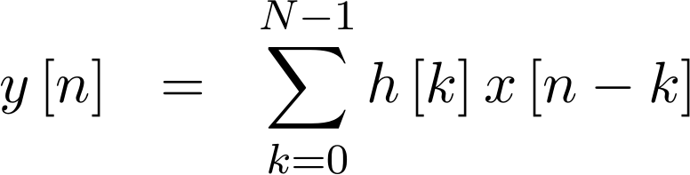 |
where there are N taps to the filter, x[n] is a sequence of input samples,
h[k] is the sequence of filter
coefficients, and y[n] is the output of the
filter.
The moving average
filter fits this form as well,
with the unique feature that all the
filter
coefficients, h[k] are all ones. This means that the multiplies are all
by one, and so they they can be removed from the
implementation.
Hence, you might draw this simplified filter as shown in Fig 2, without the multiplies.
 |
Formally, we might write this as,
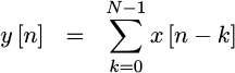 |
With this simplification, the filter has turned into nothing more than a summation of a set of input values made on every clock tick.
Even in this form, we’re not ready to implement this
filter yet.
Instead, consider what would happen if we subtracted two of these y[n]
values from each other. You can see this conceptually in Fig 3.
 |
Did you catch that? The difference between two adjacent outputs of our
filter, y[n]-y[n-1] is given by the difference between two input samples,
x[n]-x[n-N].
Mathematically, we could write this as,
 |
This subtle change in formula, from the generic formula for a convolution to the one above, will spare us a lot of logic–allowing us to use a running accumulator and a block RAM instead of hardware multiplies and a lot of flip-flops.
Further, despite this formula referencing y[n-1], it is not an
IIR filter.
Careful design will keep it from becoming one.
Let’s look at how we might implement this filter.
The Basic Equations
A very quick, though incomplete, draft of this algorithm might look like:
always @(posedge i_clk)
if (i_ce)
begin
	// Write the incoming sample to memory
	mem[wraddr] <= i_sample;
	wraddr <= wraddr + 1'b1;

	// Read the x[n-N] value from memory
	memval <= mem[rdaddr];
	rdaddr <= rdaddr + 1'b1;

	// Subtract x[n-N] from the incoming sample, x[n]
	// sub = x[n] - x[n-N]
	sub <= (i_sample - memval);

	// Add the result to the last output
	// y[n] = y[n-1] + sub = y[n-1]+x[n]-x[n-N]
	acc <= acc + sub;

	// rounded() is shorthand for what we wish to do
	// but not really valid Verilog
	o_result <= rounded(acc);
end
Walking through this implementation, our first step was to write this
new sample to memory, and update our write pointer. At the same time, we
read the value out from N samples ago, and updated our read pointer.
We then subtracted the value we read from memory, memval also known as
x[n-N], from the new value, i_sample or x[n], we just received. The
result of that subtraction was then added into our accumulator, y[n], just
like we discussed in the last section. The final step was to
round
the output to the desired number of bits and we were done.
You’ll find by the end of this article that our finished algorithm, is not going to be all that much more complex than the algorithm above, although you may also find that it doesn’t look much like the algorithm above.
Reset
The first problem with our first attempt is making certain that the
the filter
has a proper initial value. One mistake in the accumulator, one mistake
that gets y[n] wrong, and
this filter
might be turned into an
IIR filter with
an unwanted DC offset. To keep that from happening, let’s create a reset
capability so that we can guarantee the filter starts in a known configuration.
Specifically, at the time of reset, the accumulator must be set to zero,
as with any intermediate calculation values, such as sub and memval.
The other thing we’ll need to pay attention to is the memory. One difficulty when using block RAM, as with all memories I know of, is that there’s no circuitry for initializing all of our memory at once. Instead, we’ll “pretend” the memory is zero for a number of clocks following a reset, and then we’ll use the memory as normal.
Hence, we’ll need to modify our code such as,
always @(posedge i_clk)
if (i_reset)
begin
	acc <= 0;
	full <= 1'b0;
	sub  <= 0;
	wraddr <= 0;
	rdaddr <= -navg;
end else if (i_ce)
begin
	wraddr <= wraddr + 1'b1;
	rdaddr <= rdaddr + 1'b1;
	//
	full <= (full)||(rdaddr == 0);
	if (full)
		// Value read from memory is valid
		sub <= i_sample - memval;
	else
		// Value read from memory was never initialized
		// We'll assume here that it is zero
		sub <= i_sample;

	acc <= acc + sub.
end
This creates a new value, full, which we can use to determine whether the
memory value is valid or not.
These are the big broad-brush differences between the quick draft above, and what we’re about to present below. Our next step, then, will be to build our final algorithm.
The Actual Algorithm
Let’s now use the lessons from above to build our verilog algorithm. Feel free to examine the final code here, as you follow along below.
As a step number one, we’ll make this
filter
as generic as we can. To do that, we’ll parameterize our input width,
IW, and output width, OW. Further, we’ll parameterize the number of
averages allowable, which we shall controll by the log (based two) of the
maximum number of averages, LGMEM. This will allow us to average by
any amount between 1 and (1<<LGMEM)-1.
parameter	IW=16,		// Input bit-width
		LGMEM=6,	// Size of the memory
		OW=(IW+LGMEM);	// Output bit-width
Hence, if you want to average fifty-five 16-bit values together, you’d set IW
to 16 and LGMEM to 6. If you want an output without any
rounding,
then the output width, OW,
needs to be set to
the input width plus the log of the number of averages. In the example of
averaging fifty-five 16-bit items together, this means we’d need an output
width of 16+6, or OW=22. Any fewer output bits than that will require
rounding
the internal result to the desired number of output bits.
We’ll also allow the number of averages to be configurable as well–or not,
if the FIXED_NAVG parameter is set. If FIXED_NAVG is set, then the number
of averages will be fixed, and set by an INITIAL_AVG parameter.
parameter [0:0]	FIXD_NAVG=1'b0;	// True if number of averages is fixed

// Always assume we'll be averaging by the maximum amount, unless told
// otherwise.  Minus one, in two's complement, will become this number
// when interpreted as an unsigned number.
parameter [(LGMEM-1):0]	INITIAL_AVG = -1;
If FIXED_NAVG is not set, we’ll allow the user to set the number of averages
they want. However, because of the dependence of the feedback relationship,
y[n] on y[n-1], we’ll insist that the number of averages must not change
except on an i_reset signal.
wire	[(LGMEM-1):0]	w_requested_navg;
assign w_requested_navg = (FIXED_NAVG) ? INITIAL_NAVG : i_navg;
As we’ll see later, the only part of our algorithm that depends upon this number of averages is the initial/reset value of the memory read address. For this reason, we won’t store the value in a register. We’ll come back to this later when we discuss the read address.
That brings us to the logic required for accessing memory–both writing and then reading. Of these two, the write address is simple: we’ll start writing to the first address of memory (address zero) on our first data sample, and then rotate through memory locations from there.
initial	wraddr = 0;
always @(posedge i_clk)
	if (i_reset)
		wraddr <= 0;
	else if (i_ce)
		wraddr <= wraddr + 1'b1;
What that means, though, is that we have to implement the time difference
between the initial value and the value N samples ago using the read
memory address. We’ll do so by initializing the read address to the negative
number of averages.
initial	rdaddr = 0;
always @(posedge i_clk)
	if (i_reset)
		rdaddr <= -w_requested_navg;
	else if (i_ce)
		rdaddr <= rdaddr + 1'b1;
As with the write address, we increment the read address on every sample clock.
Following the address calculation, we’ll write out incoming sample to memory, and read our delayed sample from memory as well.
always @(posedge i_clk)
	if (i_ce)
		mem[wraddr] <= i_sample;

// ...

initial	memval = 0;
always @(posedge i_clk)
	if (i_ce)
		memval <= mem[rdaddr];
So far, this is all straightforward. Other than initial values, we haven’t
really deviated from our initial draft above. However, things get a little
trickier when adding the input sample to this logic. In particular, if we
want our input value to be aligned with the output of the memory read, memval,
associated with x[n-N], then we’ll need to delay the input by one sample.
It’s not really that obvious why this would be so. Why does the input need to be delayed by a sample? The answer has to do with pipeline scheduling. So, let’s look at how the internal values within our algorithm get set on subsequent clocks, as shown in Fig 4.
 |
This figure shows a list of all of our internal registers, binned within the
clocks they are set within–starting on the clock before a particular sample,
i_sample[t], is provided, t-1 until four clocks later at t+4. Hence, since memval depends upon rdaddr, it
shows in the clock following the one when rdaddr gets set. Likewise, since
the memory is set following the write address being set, mem[wraddr] gets
set following wraddr.
While our presentation through the
code below
is going to be in chronological order, from time t through t+4, the chart
above was built/scheduled backwards. o_result is the
rounded
version of acc. It took
one clock to calculate. acc is the sum of the last accumulator and the
result of the subtraction, sub. Further, we know that we want to subtract
our new input value from the last memory value, memval, etc.
So why do we have the register preval in this pipeline chart? It doesn’t
seem to do anything, so why is it there?
The answer is simple: we needed to delay the input by one clock in order to get it to line up with the memory that was just written and then read.
For example, let’s suppose we only wished to average one
element–a pass-through filter. Hence, we’d want to add
our new value, x[n], and subtract the prior value, x[n-1], delayed by only
one clock. Given that’s what we want to do, let’s follow that new value through
this pipeline schedule in Fig 5 below.
 |
i_sample[t-1] shows up at time t-1, and gets written into memory,
mem[wraddr], at time
t. It can then be read at time t+1 into memval, and then subtracted
from the new value at t+2 to create sub. This time, t+2, is the earliest
the last value can be read back from memory. This is also the time when we
need our new value, x[n]–one clock after it shows up. To get the new sample
value from when it is given to us into this clock period, we need to delay it
by a single cycle, placing it into preval for that purpose.
The logic necessary to do this is trivial–unlike the reasoning behind it above.
initial	preval = 0;
always @(posedge i_clk)
	if (i_reset)
		preval <= 0;
	else if (i_ce)
		preval <= i_sample;
The other thing we’re going to need to know, at the same time we want to
know the value we just read from memory, is whether we’ve written enough
times to the memory for the values read out of the memory to be valid. I’ve
chosen to call this full, to indicate that the tapped-delay line memory has
been filled.
Since we initialized the write address at zero, and then wrote to the zero address in our first clock, we know that the value read from memory will be valid as soon as we read from the zero address.
initial	full   = 1'b0;
always @(posedge i_clk)
	if (i_reset)
		full <= 0;
	else if (i_ce)
		full <= (full)||(rdaddr==0);
We’ve now set all of the values shown in the time t+1 column from Figs 4 and 5
above, so we’ll move on to the next clock. In this clock, we’ll subtract
the sample falling off the end of our average list from our new sample. We’ll
place this result into sub.
initial	sub = 0;
always @(posedge i_clk)
if (i_reset)
	sub <= 0;
else if (i_ce)
begin
	if (full)
		sub <= { preval[(IW-1)], preval }
				- { memval[(IW-1)], memval };
	else
		sub <= { preval[(IW-1)], preval };
end
The rest is simple. We add this difference to our accumulated value, creating
our filter’s
output value, y[n].
initial	acc = 0;
always @(posedge i_clk)
	if (i_reset)
		acc <= 0;
	else if (i_ce)
		acc <= acc + { {(LGMEM-1){sub[IW]}}, sub };
The final stage of our pipeline
rounds
our filter’s
outputs to the number of bits requested by the parameter, OW.
generate
if (IW+LGMEM == OW)
	// No rounding required, output is the acc
	assign	rounded = acc;
else if (IW+LGMEM == OW + 1)
	// Need to drop one bit, round towards even
	assign	rounded = acc + { {(OW){1'b0}}, acc[1] };
else // if (IW+LGMEM > OW + 1)
	// Drop more than one bit, rounding towards even
	assign	rounded = acc + {
			{(OW){1'b0}}, acc[(IW+LGMEM-OW)],
			{(IW+LGMEM-OW-1){!acc[(IW+LGMEM-OW)]}} };
endgenerate
Once we are done rounding the output value, we’ll take an extra clock stage to deal with any delay associated with rounding.
always @(posedge i_clk)
	if (i_reset)
		o_result <= 0;
	else if (i_ce)
		o_result <= rounded[(IW+LGMEM-1):(IW+LGMEM-OW)];
While we might’ve skipped this delay if we didn’t need to drop any bits, doing so would cause our filter to have a different delay depending on how it was configured. Rather than deal with that maintenance headache, the result is always delayed (rounded or not) by one clock here.
Performance
The frequency response of a moving average filter is well known. It’s easy enough to calculate that it makes a good assignment for the beginning student. It’s given by,
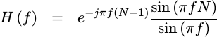 |
If you examine this response, it’s really not that great. At best, you can get a stopband of -13 dB from this filter. That’s better than the -6dB stopband from our FM example above, but still a far cry from the -70dB we might like.
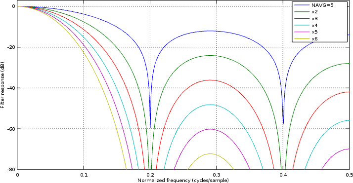
On the other hand, if you cascade M filters
of this type together, you can get a much deeper
stopband.
To illustrate this,
Fig 6 below shows, in blue, the response of a
moving average
filter
that averages five adjacent values together. The other lines on the chart show
what happens after cascading
this filter
with itself two, three, four, five, or six times.
 |
The Octave code used to create this figure can be found here.
There are two important things to notice from this figure. First, the
stopband
of the filter, when cascaded, can get very deep. After cascading six of
these together, the
stopband
is -78 dB–pretty impressive. The second thing to notice is that the
“passband”
is no longer flat. As a result, we’ll need to follow
this filter
with another one to clean up any distortion of our signal of interest.
Conclusion
While a moving average filter is a far cry from a well-designed low-pass filter, it’s also a very simple filter to implement. From an engineering trade-off standpoint, this simplicity makes it a very attractive component for dealing with many DSP requirements on an FPGA.
We’re not done with our lessons on digital filtering, though. I’ve still got plans to discuss symmetric filters, half-band filters, Hilbert transforms, and more. Further, I’d like to discuss not only their high speed implementations, but also some slower implementations that would be appropriate for those designs where there are many clocks between input samples.
Even at that, we’re not done, since the filter above, when cascaded with itself any number of times and followed by a downsampler, can be built without needing a block RAM.
We are also going to want to discuss how to go about proving that these filters work. What sort of test bench is appropriate for testing digital filters?
These, however, are lessons still to come.
Lo, this only have I found, that God hath made man upright; but they have sought out many inventions. (Eccl 7:29)