Measuring AXI latency and throughput performance

Performance.

Why are you using an FPGA? Performance.

Why are you building an ASIC? Performance. Low power, design security and size may also play a role here, but performance is still a big component.

Frankly, if you could do it some other, cheaper way, you’d do it the cheaper way. Digital logic design isn’t easy, and therefore it’s not cheap.

That endless persuit of more and better performance forms the backdrop for everything we will be discussing today. Specifically, you’ll never have good performance if you cannot measure your performance.

So, today, let’s talk about measuring the performance of the interface between an AXI master and slave.

Before diving into the topic, though, let me just share that this is an ongoing project of mine. I’ve now gone through several iterations of the measures I’ll be presenting below. Yes, I’m becoming convinced of their effectiveness–or I wouldn’t be writing. Well, that’s not quite true. I was going to present a preliminary draft of these measures–but I think what I have now is even better than that. So, today, we’ll look at what these measures are, and then use them to tell us something about how effective a particular bus structure is.

With that as a background, let’s dive right in.

AXI Performance Model

Fig 1. Connecting the AXI Performance monitor

My goal is to be able to attach to any AXI link in a system a performance monitor. This is a simple Verilog module with an AXI-lite control interface that monitors a full AXI interface. A simple write to the performance monitor will start it recording statistics, and then a second write at some later time will tell it to stop recording statistics. That much should be simple.

That’s not the challenge.

The challenge is knowing what statistics to collect short of needing the entire simulation trace.

First Attempt: Basic statistics

As a first pass at measuring performance, we can simply count both the number of bytes (and beats) transferred during our observation window together with the size of the window. We’ll even go one step further and count the number of bursts transferred.

To give this some meaning, let’s define some terms:

• Beat: A “beat” in AXI is one clock cycle where either WVALID && WREADY, for writes, or RVALID && RREADY for reads.

  The number of beats over a given time period, assuming the bus is idle at both the beginning and ending of the time period, should also equal to the sum of (AWLEN+1)s every time AWVALID && AWREADY for writes, or alternatively the sum of (ARLEN+1)s on every cycle that ARVALID && ARREADY.

• Burst: A “burst” is a single AXI request. These can be counted by the number of AWVALID && AWREADY cycles for writes, or ARVALID && ARREADY cycles for reads.

  As with beats, there are other measures we could use to count bursts. For example, we might also count WVALID && WREADY && WLAST or BVALID && BREADY cycles when counting write bursts, or RVALID && RREADY && RLAST cycles when counting read bursts.

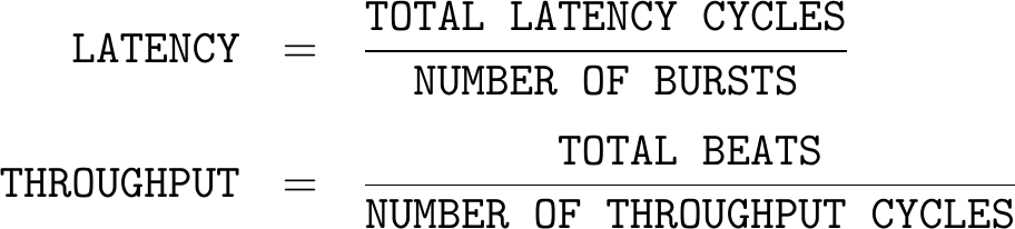
From the outputs of these first basic counters, we might calculate some simple performance measures, such as:

or

or

Now, suppose the throughput you’ve measured isn’t the throughput you were hoping for. Which module needs fixing? Should you invest your energy into updating the slave or updating the master? This suggests we might want another three measures:

• Write not ready: If the master hasn’t raised WVALID by the time AWVALID && AWREADY then the master is delinquent in providing write data. Likewise, the master is also delinquent if it fails to provide write data on every clock cycle between the first WVALID and WVALID && WLAST where WVALID is low.

  In these cases, the master is throttling the write speed. This isn’t necessarily a bad thing, but if you are monitoring AXI bus performance then you will really want to know where the bottlenecks in any transfer are coming from.

• Write back pressure: If BVALID && !BREADY are ever true, than the master is throttling a write return.

• Read back pressure: If RVALID && !RREADY are ever true, than the master is throttling a read return.

Another fairly simple, but ad hoc, measure could capture how well the AXI master and slave were able to pipeline. For that, one might just count the maximum number of outstanding bursts. The more bursts the master issues that the slave allows to be outstanding, the deeper the slave’s pipeline must be.

While these are useful metrics, there’s a lot of things these simple measures don’t capture. For example, do we really want to count against our throughput the cycles when no transfers have been requested? Wouldn’t it make more sense to therefore measure throughput instead as,

where an active clock cycle started upon some request and then ended when the request was complete?

We also discussed examples where the master was throttling our throughput. Can we expand that concept so that we can tell when the slave is throttling throughput?

Second Pass: A first order approximation

Therefore, let’s see if we can’t expand these measures into a proper first order model of transaction time. In other words, let’s see if we can model every bus transactions using a simple linear model:

The idea is that, if we can properly identify the two coefficients in this model, burst latency and throughput, then we should be able to predict how long any transaction might take. Of course, this assumes that the model fits–but we’ll have to come back to that more in detail later.

To illustrate this idea, let’s consider Fig. 2 below showing an AXI read burst.

Fig 2. Decomposing performance into two parts

Here, in this burst, you can see how it neatly divides into two parts: a latency portion between the beginning of the request and the first data beat, and then a response portion where the data beats are returned. No, the model isn’t perfect. The read throughput is arguably one beat every three cycles, but the 36% measure shown above is at least easy enough to measure and it’s probably close enough for a first attempt at AXI performance measurement.

This model, by itself, nicely fits several use cases. For example, consider the following memory speeds:

• A SPI-type NOR flash memory. In this case, the controller must first issue an 8’b command to the SPI memory. This command will be followed by a 24’b address. After command and address cycles are complete, there may be a couple of unused cycles. After all of these cycles, a SPI based flash should be able to return one byte every eight SCK cycles.

• A QSPI flash controller. If you go directly into QSPI mode via some form of eXecute In Place (XIP) option in the controller, then you can skip the command cycles. The 24 address cycles might now be accomplished in QSPI mode, leading us to 6 cycles of latency. Once the command is complete, a byte can be produced every other SCK cycle.

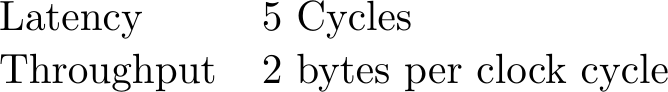
• An SDRAM. Most SDRAMs require an ACTIVATE cycle to activate a given row, followed by the memory request using that row. In my own SDRAM controller, the SDRAM can only return 16-data bits. In total, the controller has a five clock latency, followed by a throughput then of one 32-bit word every other clock cycle.

• A block RAM controller. This one should be easy, no? In the case of a block RAM, you have everything working to your advantage. However, Xilinx’s AXI block RAM controller requires 3 cycles of latency per burst.

  My own block RAM controller is a bit different. It pipelines requests. As a result, the latency will be hidden during subsequent accesses. So, for this one we might write:

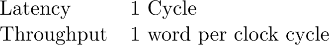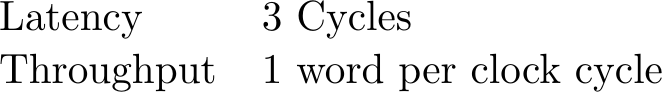
• Interconnect. This is one of the things I really want to measure. From what I know of my own interconnect, I expect three cycles of (pipelined) latency per burst–the first is used to decode the address, and the second two are required by the AXI protocol.

That’s what I think it should achieve. But … does it?

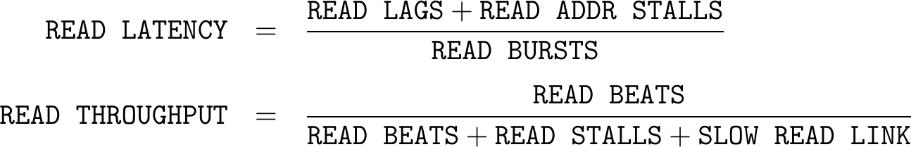
Still, the model seems to fit several potential slave interactions–enough so that it looks like it might be useful. Therefore, let’s see if we can build a linear AXI performance model. Let’s start these efforts by considering Fig. 2, shown again below, as a reference. This time, however, our goal is going to be to categorize every clock cycle used by this transaction so that we can then draw conclusions about the performance of the bus at a later time.

Fig 3. Decomposing performance into two parts

Using this model, we’ll define latency as the time following when the master first raises ARVALID for reads until the first RVALID is available. Latency will be expressed in clock cycles per burst. We’ll then define throughput as the number of beats transmitted divided by the time between the first RVALID and the last RVALID && RREADY && RLAST. Unlike latency, however, we’ll define throughput in terms of a percentage. Of those clock cycles between RVALID and the end of RVALID && RREADY && RLAST, the throughput will be defined as the percentage of clock cycles in which a beat of data was transferred.

Using these metrics, the best AXI slave will have a latency of zero, and a throughput of 100%–assuming the master doesn’t slow it down with any back pressure.

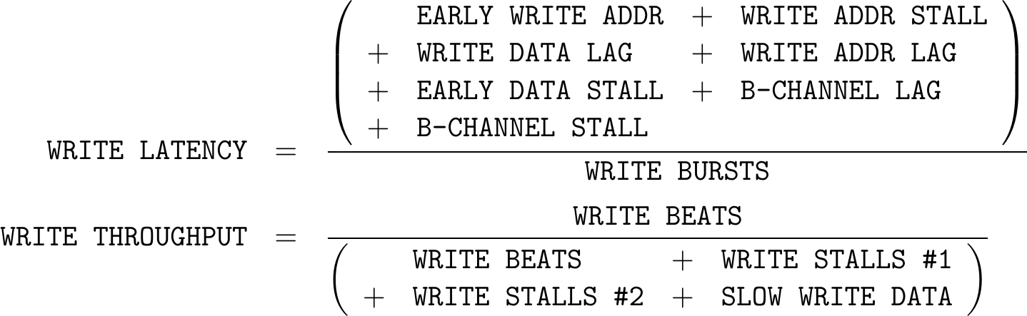
We’ll use a similar model for writes, although we will need to modify it just a touch as shown in Fig. 4 below.

Fig 4. Decomposing write performance into latency and throughput components

Fig 5. How shall write latency be defined?

In the case of writes, latency comes in two parts. There’s the latency between the first AWVALID and the first WVALID && WREADY. Once WVALID && WREADY have been received, the time from then until WVALID && WREADY && WLAST will be a measure of our throughput. After measuring write throughput, there will then at least one additional cycle of latency until BVALID && BREADY.

At a first glance, this model seems simple enough: count the number of latency cycles and the number of throughput cycles. Then, with an appropriate scale factor, we should be able to calculate these coefficients:

Let’s try it out and see what happens!

Data Collection Methodology

Our basic method will be to examine evey AXI signal, on a clock by clock basis, and to bin each cycle, as I illustrated in Fig’s 3 and 4 above. We’ll then count the number of clock cycles in each of a set of various categories. To make this work, though, we’re going to need to make certain that no clock cycle is counted in more than one bin. Let me therefore present the two bin classifications that I am (currently) using.

First, let me start with the read classification, since that one is easier to follow. Fig. 6 below shows a table, allowing every AXI beat on the read channels to be classified.

Fig 6. Categorizing AXI read cycles

In this table, empty boxes represent “don’t care” criteria.

Those who are familiar with AXI will recognize the ARVALID, ARREADY, RVALID and RREADY signals heading up this table. These are to be expected. The two new flags in this chart capture the state of a transaction. The bursts in flight flag measures whether or not RVALID has been true for a given burst so far, but RVALID && RLAST has not yet been true. Hence, if a burst is in flight but the data isn’t (yet) available, then we have a throughput problem. This is illustrated by the “Slow read link” name above, and by the SL cycles in Fig. 3 above. The second measure is whether or not a burst is outstanding. An outstanding burst is one for whom ARVALID && ARREADY has been received, but for which RVALID has yet to be asserted. Therefore, any time a burst is outstanding, but before the return is in flight, we’ll call that clock cycle a latency cycle. These are the LG cycles in Fig. 3 above.

Now, if we’ve done this right, then all of the cycles above will add up to the total number of cycles from capture start to capture end. This will allow us some additional measures as well. For example, what percentage of time is the bus being used, or similarly what percentage of time is being spent waiting for the return leg to start responding?

What can these bins tell us?

• READ IDLE: This tells us how busy the bus is. This is simple enough. If you want to move a lot of information but spend the majority of time with the bus idle, then maybe you want to consider using an AXI DMA instead of a memcpy().

• READ BEAT: This one of the most important bins, since it tells us how much data we are putting through the interface. In a busy bus, you will want the READ BEAT bin to occur as often as you can–simply because it means you are then getting high throughput.

• READ STALL: This is the back pressure measure. This is due to the master telling the slave that it’s not ready to receive data. A good master won’t do this, but there are times when back pressure is required: clock domain crossings, waiting for return arbitration in the interconnect, etc.

• SLOW LINK: This is our measure of the read data not being available. Those examples above, such as from the SPI flash, that didn’t achieve full bus performance would’ve been due to a slow link after the first clock cycle of the burst. In this case, the slave has started to provide read data, and so the first beat of the read burst has been returned, but the slave doesn’t (yet) have the data ready for the next beat of the burst. Unlike the read stall, which was the master’s problem, a slow link is the fault of the slave. This doesn’t necessarily mean the controller is at fault, it might just be that the hardware can only go so fast in the first place.

• READ LAG: This measure counts the beats between ARVALID && ARREADY and the first RVALID. This is the component we would normally think of as the bus latency.

• READ ADDR STALL: Counts the number of beats where ARVALID && !ARREADY. This can happen for a lot of reasons–notably when a burst is already outstanding and the slave can’t handle more than one burst at a time. For this reason, we only count read address stalls when nothing else is outstanding. That makes this an indication of a poor AXI implementation in the slave–typically indicating that the slave doesn’t allow ARREADY to idle high, but in some cases (like Xilinx’s IPIF interface bridge) it might simply be an indication that the slave is working on the burst already but just hasn’t let the master know that it has accepted the request.

• READ ADDR CYCLE: This simply counts the first ARVALID && ARREADY of every burst. It’s subtly different from a read burst count, simply because we only count ARVALID && ARREADY when the interface is otherwise idle.

From these measures, we should be able to calculate:

You may have noticed that this categorization prioritizes certain conditions over other possibilities. For example, the ARVALID and ARREADY bins are both don’t care bins when RVALID is high. That’s because the link speed is, at that time, driven by the speed of the return. Additional packets that arrive (should) go into a pipeline somewhere in the processing queue. We don’t pay attention to them at all–at least not until they start to impact the return.

Indeed, our choice here becomes one of the many decisions that need to be made when trying to measure AXI performance, decisions which subtly prioritize performance in one part of the spectrum perhaps to the detriment of measuring performance in other cases. Our choices have limited the bus to one of six possible bus cycles on every clock.

The problem only gets worse when we get to the write channel. In the case of the write channel, we have three separate channels that need to be somehow prioritized: AW*, W*, and B*. Worse, AXI imposes no particular order between AW* and W*. How then shall we allocate blame between master and slave, or rather, how shall we then tally meaningful performance metrics in this environment?

Fig. 7 below shows you my solution to this problem. Yes, it is much more complicated than reads are, as you can see by the existence of fifteen bins versus the seven we had before.

Fig 7. Categorizing AXI write cycles

Let me take a moment, again, to explain the new columns. The first one, outstanding address, is a flag that will be true between the first AWVALID && AWREADY and the BVALID && BREADY associated with the last outstanding transaction. It indicates that there’s an outstanding write address request, and therefore an outstanding write burst, that has not yet completed. The second one is similar. This one will be true between the first WVALID && WREADY and the last BVALID && BREADY. These two flags are useful when trying to figure out the synchronization between the two channels. For example, if the outstanding address is true but the outstanding write data is not, then the address arrived before the write data. The write in progress flag is very similar to the bursts in flight flag from the read side. This flag will be true from the first WVALID signal until its associated WVALID && WREADY && WLAST.

As with the read channel, we are prioritizing throughput over all other conditions. For this reason the first write categories all contain WVALID. These are prioritized over BVALID or even AWVALID cycles.

Let’s examine these categories in more detail.

• WRITE BEAT: This is simply a count of every write beat.

• EARLY WRITE BEAT: This is a special category of write beat. Unlike our other categories, this one duplicates some of the counts of one other category, notable the WRITE BEATs count above. I’ve added this one to the mix so that we can capture the concept of the write data showing up before the address. (This didn’t happen in any of my tests …)

• WRITE STALL #1: There are two different types of write stalls that we recognize. In both cases, WVALID && !WREADY will indicate a write stall. In this first case, AWVALID && AWREADY has already taken place, so that we now have an outstanding burst that this stalled data is assigned to.

  This is what you might think of as a normal write stall. It’s driven by the slave’s inability to keep up with the masters data rate.

• WRITE STALL #2: Like the write stall above, this is also a measure of the total number of write stalls. Where this measure differs is that this stall captures those cases where a write is in progress already. In order to differentiate this from the stall above, these stalls are only in the case where the write address has not shown up yet.

  Since most slaves can’t do anything but buffer write data until the associated address shows up, stalls here may be more a reflection of slave stalling until the address is available, verses the slave stalling due to a true lack of throughput. Once the slave’s buffer fills up, these stalls are really a problem with the master not providing AWVALID–not with any capability in the slave.

  In my own AXI designs, the slave’s write buffer tends to be a simple skid buffer, so once you get past the first beat the slave will always need to stall until the address is available.

• SLOW WRITE: In this case, an address has been provided to the slave in addition to the first write beat of data. The problem here is that the master has been unable to keep the slave’s write data channel full.

  I generally design my AXI masters to avoid issuing an AWVALID until they can keep WVALID full throughout the whole burst. The problem with issuing AWVALID early, and then not having the data when you need it, is that it can otherwise lock up the channel for all other users.

• EARLY WRITE ADDR: This is the case where the write address shows up before the data. There’s nothing wrong with this per se, except that the slave can’t yet act on this address until the data (eventually) shows up.

• WRITE ADDR STALL: As you might expect, this is the case where AWVALID && !AWREADY. However, in this case, there is a catch. We’re only going to count this as a write address stall if the channel isn’t otherwise busy. Once a burst has started, the slave may need to stall the AW* channel simply because it might not be able to handle more than one burst at a time. By excluding those cases, we’re instead catching any examples of a slave that doesn’t use a skid buffer.

• WRITE DATA LAG: Once the write address has been accepted, any lag between the address and the data is going to add to our latency measure. We’ll call this the write data lag. If you look at Fig. 4 above, you’ll see that there is one beat marked LG. This would be a beat of write data lag.

• WRITE ADDR LAG #1: If the write data shows up before the address, we again have a latency situation–this time, though, with the data ahead of the address. What makes this latency measure unusual is that the entire write burst has been received–since there’s no longer any write in progress.

• WRITE ADDR LAG #2: This measure is a bit more what we might expect–the first write data has shown up and so we are mid-burst, but the address hasn’t shown up yet.

• EARLY DATA STALL: It may be to the slave’s advantage to stall the data channel until after the address has been received. Indeed, you may remember that I did so in my own AXI (full) slave demo. Even though there may be good reasons for this, however, it’s still a write data stall that we’re going to need to keep track of.

• B CHANNEL LAG: That brings us to our three B* channel statistics. These are specially constructed so that they are only counted when none of the other conditions above are counted. In the case of this first measure, the B channel lag counts the case where all the data has been received but BVALID has yet to be set.

• B CHANNEL STALL: As with the B channel lag, this stall only applies once all the data has been received and no more WVALID data is incoming. This is an indication that the master is not yet able to receive a response, but that the slave has the response ready and available for the master to consume.

• B CHANNEL END OF BURST: Just for completion, we also need to keep track of the BVALID && BREADY cycles when nothing else is happening.

• WRITE IDLES: This finishes out the count of all cycles, so that we’ve somehow categorized every clock cycle–idle cycles, data cycles, and lag cycles.

Put together, we should be able to identify latency and throughput.

Ad hoc Measures

Just for good measure, I added a couple ad hoc measures to this list to see if I could get even more insight into how a given link was working.

Here are some of the additional and extra read measures I’m currently keeping track of:

• Maximum read burst size. In general, a slave can often optimize data handling if it knows where the next request is coming from, or perhaps if it knows ahead of time that the data will be read in order. The larger the burst size, the easier it can be to do this. Therefore, knowing the maximum burst size is a useful measure of how well burst reads are being employed.

  This would certainly be the case when interacting with Xilinx’s block RAM controller. Since it doesn’t pipeline requests, you would need large burst requests to get good throughput numbers from it.

• Maximum number of ID’s that have bursts in flight at any given time. This is a measure of the out of order nature of the return channel. The more out of order the read channel is, the more burst ID’s that may be outstanding at any given time.

  Unfortunately, my own AXI interconnect doesn’t yet forward requests downstream from multiple AXI masters. Instead, it will only allocate one master to a slave at a time. This limits the maximum number of outstanding burst ID’s to those created by a single master alone. No, it’s not as powerful as an AXI interconnect can be, but it does work, and it is open source (Apache 2). Perhaps when I finish my current contract I’ll have a chance to come back to it and finish adding this feature in. Until then, our tests below won’t be able to register much here.

Likewise, here are some extra write measures I’m going to keep track of as well:

• Write bias. This is designed to capture the extent to which the AW* channel shows up before the W* channel. Hence, if AW* is ahead of the W* channel I add one, otherwise if W* is ahead of AW* I subtract one.

• The maximum number of outstanding write bursts at any given time. This is intended to provide an indication of the allowed AXI pipeline depth.

• Maximum write burst size. This is a measure of the extent to which bursts are being used. It’s a compliment to the ratio of write beats to write bursts.

Whether or not any of these measures will be valuable is still something I’m looking into.

Adjusting the EasyAXIL design

This is the section where I typically present a design of some type. In this case, I’ll be sharing the AXI performance monitor design I’ve been working with.

This particular design is now one of many AXI designs I’ve built following the EasyAXIL prototype. The EasyAXIL AXI-lite prototype is just really easy to work with, while also achieving good performance on an AXI-lite bus. Because this design repeats the signaling logic from the EasyAXIL design, I’ll skip that portion of the presentation below. Feel free to check out the EasyAXIL article for more information on how the AXI-lite signals are generated. For now, it’s important to remember that the internal axil_write_ready signal indicates that we are currently processing a beat of write information whereas the internal axil_read_ready signal indicates we are reading a beat of information. In both of these cases, the address will be in awskd_addr and arskd_addr respectively after removing the (unused) least significant address bits. Similarly, the write data will be found in wskd_data and wskd_strb respectively.

Speaking of writes, let’s just look at how this core handles writes to its AXI-lite interface. In general, there are only three registers controlled by the write interface:

• clear_request: If the user ever sets this register, we’ll automatically reset all of our counters. The reset will complete once the bus returns to idle.

• start_request: This register requests we start accumulating AXI data. The signal will remain high until the bus becomes idle and any (potentially) pending clear_request has completed. At that time the design will start accumulating its statistics.

  Waiting for the bus to become idle is a necessary requirement, lest our statistics be incomplete. Beware, however, that our performance monitor might be downstream of the link we are monitoring. For example, what if this performance monitor is attached to a CPU via its data bus connection? In such cases, even the request to start monitoring would then only be provided in the middle of a bus transaction! This makes idle tracking all the more important.

• stop_request: Once data acquisition is complete, a stop request requests we stop accumulating data. As with the start_request, the stop_request signal will be sticky and remain set until the bus becomes idle.

There is the possibility that our bus utilization counters will overflow. I currently have these counters set to a maximum of 256 outstanding bursts. Overflowing this number seems like it would be highly unusual. However, if this ever happens, this performance measurement design will of necessity lock up until the next bus reset. By “lock up”, I mean that it will refuse to make further measurements. We’ll come back to this again in a moment. For now, just know that if this ever happens you may need to increase the size of the counters used to keep track of the number of outstanding bursts–not the number of beats received or outstanding, but the number of outstanding bursts.

Now, here’s how we use these flags together:

	always @(posedge S_AXI_ACLK)
	begin
		if (idle_bus)
			clear_request <= 1'b0;
		if (!clear_request && idle_bus)
		begin
			start_request <= 0;
			stop_request <= 0;
		end

These three flags are all self clearing. Therefore, the first thing we’ll do is to clear them. The clear_request can complete only when the bus is idle–otherwise our counters will be all messed up. Similarly, start and stop requests are just that: requests. They remain requests until the bus is both idle and any pending clearing request is complete. Once the bus becomes idle, then accumulation can start or stop.

The next step is to handle any write requests.

		if (axil_write_ready)
		begin
			case(awskd_addr)
			5'h1f:	if (wskd_strb[0]) begin
				// Start, stop, clear, reset
				//
				clear_request <=  (clear_request && !idle_bus)
					|| (wskd_data[1] && !wskd_data[0]);
				stop_request  <= !wskd_data[0];
				start_request <=  wskd_data[0] && (!stop_request);
				end
			default: begin end
			endcase
		end

Note that we’re only responding to the last address in the performance monitor’s address space. Writes to bit zero of that address will either start or stop data collection. A write to bit one clears the accumulators. From this, the usage looks like: write 1 to start, 0 to stop, 2 to clear and 3 to clear and then start.

On a reset, we’ll also clear all of these request registers.

		if (!S_AXI_ARESETN)
		begin
			clear_request <= 1'b0;
			stop_request  <= 1'b0;
			start_request <= 1'b0;
		end
	end

This logic isn’t perfect, but it’s probably good enough. For example, what happens if you write a start request while the design is already running? Or if you issue a stop request before the start request completes and the design actually starts? I may come back later and adjust this logic subtly for these corner cases, but like I said, it’s probably good enough for now. (At least it won’t cause the bus to seize up, like Xilinx’s AXI-lite template does.)

The read interface for this performance monitor isn’t really all that different from many others: it’s a giant case statement depending upon the AXI address. Remember, though, when reading this case statement below, that the arskd_addr address is not the original AXI address. Bits [1:0] have been stripped off to make this a word address.

	initial	axil_read_data = 0;
	always @(posedge S_AXI_ACLK)
	if (OPT_LOWPOWER && !S_AXI_ARESETN)
		axil_read_data <= 0;
	else if (!S_AXIL_RVALID || S_AXIL_RREADY)
	begin
		axil_read_data <= 0;
		case(arskd_addr)
		5'h00: begin
			if (!active_time[LGCNT])
				axil_read_data[LGCNT-1:0] <= active_time[LGCNT-1:0];
			else
				// OVERFLOW!
				axil_read_data <= -1;
			end
		5'h01: axil_read_data <= { wr_max_outstanding,
					rd_max_outstanding_bursts,
					wr_max_burst_size,
					rd_max_burst_size };
		5'h02: axil_read_data[LGCNT-1:0] <= wr_idle_cycles;
		5'h03: axil_read_data[LGCNT-1:0] <= wr_awburst_count;
		5'h04: axil_read_data[LGCNT-1:0] <= wr_beat_count;
		5'h05: axil_read_data[LGCNT-1:0] <= wr_aw_byte_count;
		5'h06: axil_read_data[LGCNT-1:0] <= wr_w_byte_count;
		//
		5'h07: axil_read_data[LGCNT-1:0] <= wr_slow_data;
		5'h08: axil_read_data[LGCNT-1:0] <= wr_stall;
		5'h09: axil_read_data[LGCNT-1:0] <= wr_addr_lag;
		5'h0a: axil_read_data[LGCNT-1:0] <= wr_data_lag;
		5'h0b: axil_read_data[LGCNT-1:0] <= wr_awr_early;
		5'h0c: axil_read_data[LGCNT-1:0] <= wr_early_beat;
		5'h0d: axil_read_data[LGCNT-1:0] <= wr_addr_stall;
		5'h0e: axil_read_data[LGCNT-1:0] <= wr_early_stall;
		5'h0f: axil_read_data[LGCNT-1:0] <= wr_b_lag_count;
		5'h10: axil_read_data[LGCNT-1:0] <= wr_b_stall_count;
		5'h11: axil_read_data[LGCNT-1:0] <= wr_b_end_count;
		//
		5'h12: begin
			// Sign extend the write bias
			if (wr_bias[LGCNT-1])
				axil_read_data <= -1;
			axil_read_data[LGCNT-1:0] <= wr_bias;
			end
		// Reserved for the first write lag
		// 5'h13: axil_read_data[LGCNT-1:0] <= wr_first_lag;
		//
		5'h14: axil_read_data[LGCNT-1:0] <= rd_idle_cycles;
		5'h15: axil_read_data	<= {
				{(C_AXIL_DATA_WIDTH-C_AXI_ID_WIDTH-1){1'b0}},
				rd_max_responding_bursts };
		5'h16: axil_read_data[LGCNT-1:0] <= rd_burst_count;
		5'h17: axil_read_data[LGCNT-1:0] <= rd_beat_count;
		5'h18: axil_read_data[LGCNT-1:0] <= rd_byte_count;
		5'h19: axil_read_data[LGCNT-1:0] <= rd_ar_cycles;
		5'h1a: axil_read_data[LGCNT-1:0] <= rd_ar_stalls;
		5'h1b: axil_read_data[LGCNT-1:0] <= rd_r_stalls;
		5'h1c: axil_read_data[LGCNT-1:0] <= rd_lag_counter;
		5'h1d: axil_read_data[LGCNT-1:0] <= rd_slow_link;
		5'h1e: axil_read_data[LGCNT-1:0] <= rd_first_lag;
		5'h1f: axil_read_data <= {
				// pending_idle,
				// pending_first_burst,
				// cleared,
				28'h0, perf_err,
				triggered,
				clear_request,
				start_request
				};
		default: begin end
		endcase

		if (OPT_LOWPOWER && !axil_read_ready)
			axil_read_data <= 0;
	end

In general we’re just returning various counter values. LGCNT above is the parameterized width of the various counters. I use it to help guarantee that any unused bits are set to zero.

There are three exceptions to this rule.

The first exception is the active_time counter. This counts how many cycles the performance monitor has been actively counting. If this counter ever rolls over, then all measurements are likely suspect. (All other accumulators will have values less than this one.) For this reason, we’ll check for rollover and set this value to all ones if it ever happens. Anything less than all ones, therefore, is an indication of a valid performance measurement.

The second exception is the write bias count. This is a count of the number of times the write address shows up prior to the write data. It’s a signed number, however, since the write data might show up first. Therefore, we need to check the sign bit of this value and sign extend it as necessary.

The third exception has to do with the OPT_LOWPOWER parameter. This is an option I’ve been working with as part of an ongoing experiment to use a little bit of extra logic to force values, particularly those with a potential high fanout, to zero unless they are qualified as having some meaning or other. In this case, if RVALID isn’t also going to transition high, then let’s not allow these flip-flops to toggle either. This will lead to a later assertion that if !RVALID then RDATA must equal zero.

That’s the AXI-lite handling.

The next piece of this logic is the triggered flag. I use this to help guarantee that data are only accumulated between times when the logic is idle.

	always @(posedge S_AXI_ACLK)
	if (!S_AXI_ARESETN || clear_request)
		triggered <= 0;
	else if (idle_bus)
	begin
		if (start_request)
			triggered <= 1'b1;
		if (stop_request)
			triggered <= 0;
	end

This allows our counters to all have the general form of the active_time counter below.

	always @(posedge S_AXI_ACLK)
	if (!S_AXI_ARESETN || clear_request)
		active_time <= 0;
	else if (triggered)
	begin
		if (!active_time[LGCNT])
			active_time <= active_time + 1;
	end

This active_time counter captures the total number of clock cycles that our collection is active. This is the only counter we have that uses more than LGCNT bits–allowing us an ability to detect overflow in any of our accumulators if ever the high order of this one counter is set.

We’ll need one more control signal before diving into the gathering of statistics, and that is the flag to tell us if the bus is idle or not.

	always @(posedge S_AXI_ACLK)
	if (!S_AXI_ARESETN)
		r_idle_bus <= 1;
	else if (perf_err)
		r_idle_bus <= 1;
	else if (M_AXI_AWVALID || M_AXI_WVALID || M_AXI_ARVALID)
		r_idle_bus <= 0;
	else if ((wr_aw_outstanding
			==((M_AXI_BVALID && M_AXI_BREADY) ? 1:0))
		&& (wr_w_outstanding == ((M_AXI_BVALID && M_AXI_BREADY) ? 1:0))
		&& (rd_outstanding_bursts
			==((M_AXI_RVALID && M_AXI_RREADY && M_AXI_RLAST)? 1:0)))
		r_idle_bus <= 1;

	assign	idle_bus = r_idle_bus && !M_AXI_AWVALID && !M_AXI_WVALID
			&& !M_AXI_ARVALID;

Let me point out quickly here, to no one’s surprise I’m sure, that I’ve adopted Xilinx’s AXI nomenclature. I’ve therefore prefixed my AXI-lite slave signals with S_AXIL_, whereas the signals of the bus we are monitoring are all prefixed with M_AXI_. Hence, the check above is to determine if the bus we are monitoring is idle or not.

In general, if any valid request signal is high than the bus isn’t idle.

We’ll get to some of the counters used in this logic in a moment. For now, understand that wr_aw_outstanding is a measure of the number of bursts outstanding on the AW* channel and the other *_outstanding* counters are similarly defined.

Let’s talk about the perf_err signal for a moment. This signal indicates an unrecoverable error in the performance monitor logic.
This is the error indicating a bus idle tracking counter overflow. It’s based upon overflow measures for three counters: the number of outstanding AW* bursts, the number of outstanding W* bursts, and the number of outstanding read bursts. If any of these counters ever overflow, then we can no longer tell when the bus is idle and therefore no longer know when to start or stop measuring bus performance.

As a result, once perf_err gets set, then the bus will never return idle until the next reset.

	always @(posedge S_AXI_ACLK)
	if (!S_AXI_ARESETN)
		perf_err <= 0;
	else if (wr_aw_err || wr_w_err || rd_err)
		perf_err <= 1;

Let’s now move on to the various counters, starting with the write half of the interface.

Write Accumulators

I’m not sure that there’s necessarily a good order to present accumulators for the write transactions, so we’ll just kind of work our way through them in a seemingly pseudo-random fashion.

Our first statistic captures the maximum write burst size. This is useful for knowing to what extent burst accesses were used on a given link.

	initial	wr_max_burst_size = 0;
	always @(posedge S_AXI_ACLK)
	if (!S_AXI_ARESETN || clear_request)
		wr_max_burst_size <= 0;
	else if (triggered)
	begin
		if (M_AXI_AWVALID && M_AXI_AWLEN > wr_max_burst_size)
			wr_max_burst_size <= M_AXI_AWLEN;
	end

wr_awburst_count is a count of the number of burst requests that the design has received in total.

	initial	wr_awburst_count = 0;
	always @(posedge S_AXI_ACLK)
	if (!S_AXI_ARESETN || clear_request)
		wr_awburst_count <= 0;
	else if (triggered && M_AXI_AWVALID && M_AXI_AWREADY)
		wr_awburst_count <= wr_awburst_count + 1;

wr_beat_count counts the number of write beats, that is the number of times WVALID && WREADY are true–regardless of how much information is contained in any given beat.

	initial	wr_beat_count = 0;
	always @(posedge S_AXI_ACLK)
	if (!S_AXI_ARESETN || clear_request)
		wr_beat_count <= 0;
	else if (triggered && M_AXI_WVALID && M_AXI_WREADY)
		wr_beat_count <= wr_beat_count + 1;

In order to measure the effects of narrow bursts, we’ll keep track of how many bytes may be transmitted in total. This may well be less than the number of bytes the bus is capable of transmitting.

	always @(posedge S_AXI_ACLK)
	if (!S_AXI_ARESETN || clear_request)
		wr_aw_byte_count <= 0;
	else if (triggered && M_AXI_AWVALID && M_AXI_AWREADY)
	begin
		wr_aw_byte_count <= wr_aw_byte_count
			+ (({ 24'b0, M_AXI_AWLEN}+32'h1) << M_AXI_AWSIZE);
	end

This now captures the maximum number of bytes that may be transmitted, given the burst information. But what if the bus doesn’t set AWSIZE appropriately? The bus might contain less than a word of information in that case. Knowing how much data is contained in any given beat is an important measure, so let’s capture that by counting the number of WSTRB bits that are high in any given beat.

	always @(*)
	begin
		wstrb_count = 0;
		for(ik=0; ik<C_AXI_DATA_WIDTH/8; ik=ik+1)
		if (M_AXI_WSTRB[ik])
			wstrb_count = wstrb_count + 1;
	end

We’ll then accumulate this wstrb_count into a total write byte count.

	always @(posedge S_AXI_ACLK)
	if (!S_AXI_ARESETN || clear_request)
		wr_w_byte_count <= 0;
	else if (triggered && M_AXI_WVALID && M_AXI_WREADY)
	begin
		wr_w_byte_count <= wr_w_byte_count
			+ { {(LGCNT-C_AXI_DATA_WIDTH/8-1){1'b0}}, wstrb_count };
	end

We also need to keep track of whether or not the bus is idle from a write perspective. This is different from our regular performance counters, in that this counter is never reset by anything other than an actual bus reset.

Since there’s the potential that this counter might overflow, we’ll check for and keep track of a wr_aw_err here. If there is a counter overflow in this counter, however, ALL statistics following will be suspect. Indeed, we’d then never know when the bus is idle in order to start or stop counting. This makes this a rather catastrophic error–and one that can only ever be fixed on a reset–and only avoided by using a wider burst counter.

With that aside, let’s keep track of how many bursts are outstanding. We’ll start by looking at the AW* channel, and accumulate this value into wr_aw_outstanding. As is my custom, I’ll also use a flag, wr_aw_zero_outstanding, to keep track of when this counter is zero.

	initial	wr_aw_outstanding = 0;
	initial	wr_aw_zero_outstanding = 1;
	initial	wr_aw_err = 0;
	always @(posedge S_AXI_ACLK)
	if (!S_AXI_ARESETN)
	begin
		wr_aw_outstanding <= 0;
		wr_aw_zero_outstanding <= 1;
		wr_aw_err <= 0;
	end else if (!wr_aw_err)
	case ({ M_AXI_AWVALID && M_AXI_AWREADY,
				M_AXI_BVALID && M_AXI_BREADY })
	2'b10: begin
		{ wr_aw_err, wr_aw_outstanding } <= wr_aw_outstanding + 1;
		wr_aw_zero_outstanding <= 0;
		end
	2'b01: begin
		wr_aw_outstanding <= wr_aw_outstanding - 1;
		wr_aw_zero_outstanding <= (wr_aw_outstanding <= 1);
		end
	default: begin end
	endcase

The next step is to keep track of the maximum number of outstanding AW* bursts in a counter called wr_aw_max_outstanding. Unlike wr_aw_outstanding above, this is one of our accumulators. Therefore it gets zeroed on either a reset or a clear, and it only accumulates once we’ve been triggered.

	initial	wr_aw_max_outstanding = 0;
	always @(posedge S_AXI_ACLK)
	if (!S_AXI_ARESETN || clear_request)
		wr_aw_max_outstanding <= 0;
	else if (triggered && (wr_aw_max_outstanding < wr_aw_outstanding))
		wr_aw_max_outstanding <= wr_aw_outstanding;

We’ll now repeat these same two calculations above, but this time looking at the maximum number of bursts present on the write data channel instead of the write address channel.

As before, the first measure is independent of whether or not we have been triggered. This measure counts the number of write bursts that are outstanding. We used this above to know if the channel was idle. As such, it must always count–whether or not we are triggered, and any overflow must be flagged as an performance monitor error requiring a bus reset.

	initial	wr_w_outstanding = 0;
	initial	wr_w_zero_outstanding = 1;
	initial	wr_w_err = 0;
	always @(posedge S_AXI_ACLK)
	if (!S_AXI_ARESETN)
	begin
		wr_w_outstanding <= 0;
		wr_w_zero_outstanding <= 1;
		wr_w_err <= 0;
	end else if (!wr_w_err)
	case ({ M_AXI_WVALID && M_AXI_WREADY && M_AXI_WLAST,
				M_AXI_BVALID && M_AXI_BREADY })
	2'b10: begin
		{ wr_w_err, wr_w_outstanding } <= wr_w_outstanding + 1;
		wr_w_zero_outstanding <= 0;
		end
	2'b01: begin
		wr_w_outstanding <= wr_w_outstanding - 1;
		wr_w_zero_outstanding <= (wr_w_outstanding <= 1);
		end
	default: begin end
	endcase

We’ll also keep track of the maximum number of outstanding bursts on the W* channel.

	initial	wr_w_max_outstanding = 0;
	always @(posedge S_AXI_ACLK)
	if (!S_AXI_ARESETN || clear_request)
		wr_w_max_outstanding <= 0;
	else if (triggered)
	begin
		if (wr_w_outstanding + (wr_in_progress ? 1:0)
					> wr_max_outstanding)
			wr_w_max_outstanding <= wr_w_outstanding
						+ (wr_in_progress ? 1:0);
	end

Note that this calculation depends on the wr_in_progress flag that we alluded to above. We’ll get to that in a moment. We need that wr_in_progress flag here in order to include the burst that is currently in process when calculating this maximum number of outstanding values.

The next question is, what is the total maximum number of all outstanding bursts? This number is a bit trickier, since the maximum number might take place on either the AW* channel or the W* channel. Therefore, let’s take a second clock to resolve between these two possible maximum values, and place the absolute maximum burst count into wr_max_outstanding.

	always @(*)
	begin
		wr_now_outstanding = wr_w_max_outstanding;
		if (wr_aw_max_outstanding > wr_now_outstanding)
			wr_now_outstanding = wr_aw_max_outstanding;
	end

	initial	wr_max_outstanding = 0;
	always @(posedge S_AXI_ACLK)
	if (!S_AXI_ARESETN || clear_request)
		wr_max_outstanding <= 0;
	else if (triggered)
	begin
		if (wr_now_outstanding > wr_max_outstanding)
			wr_max_outstanding <= wr_now_outstanding;
	end

We’ve alluded to the wr_in_progress signal several times now. This is the signal used in Fig. 7 above to indicate if we were mid-write data packet. As with many of the other signals, this one is fairly simple to calculate–it’s just a simple 1-bit signal.

	initial	wr_in_progress = 0;
	always @(posedge S_AXI_ACLK)
	if (!S_AXI_ARESETN)
		wr_in_progress <= 0;
	else if (M_AXI_WVALID)
	begin
		if (M_AXI_WREADY && M_AXI_WLAST)
			wr_in_progress <= 0;
		else
			wr_in_progress <= 1;
	end

In this definition, there are two important conditions. The first one is WVALID but not WREADY && WLAST. In this case, a burst is beginning or in progress. However, if WREADY && WLAST then we’ve just received the last beat of this burst and so there’s no longer any write data burst in progress.

The biggest group left, however, is the group we introduced in our write signal table in Fig. 7 above. For brevity, we’ll ignore the basic reset and setup logic for these register counters.

	initial	begin
		// Reset these counters initially
		// ...
	end
	always @(posedge S_AXI_ACLK)
	if (!S_AXI_ARESETN || clear_request)
	begin
		// Reset the counters on a reset or clear request
		// ...
	end else if (triggered)

Once we ignore this setup, we get directly to the meat of counting our critical performance measures. These should read very similar to our table above in Fig. 7. Indeed, the casez expression below turns the logic essentially into Fig. 7, so that when building these expressions I often cross referenced the two to know that I was getting them right.

	casez({ !wr_aw_zero_outstanding, !wr_w_zero_outstanding,
		wr_in_progress,
		M_AXI_AWVALID, M_AXI_AWREADY,
		M_AXI_WVALID,  M_AXI_WREADY,
		M_AXI_BVALID,  M_AXI_BREADY })
	9'b0000?0???: wr_idle_cycles   <= wr_idle_cycles   + 1;
	//
// Throughput measures
	9'b1?1??0???: wr_slow_data <= wr_slow_data  + 1;
	9'b1????10??: wr_stall     <= wr_stall      + 1;	// Stall #1
	9'b0?1??10??: wr_stall     <= wr_stall      + 1;	// Stall #2
	//
	9'b0??0?11??: wr_early_beat<= wr_early_beat + 1;	// Before AWV
	// 9'b?????11??: wr_beat   <= wr_beat       + 1;	// Elsewhere
	//
// Lag measures
	9'b000110???: wr_awr_early  <= wr_awr_early + 1;
	9'b000100???: wr_addr_stall <= wr_addr_stall + 1;

	9'b100??0???: wr_data_lag   <= wr_data_lag   + 1;
	9'b010??0???: wr_addr_lag   <= wr_addr_lag   + 1;
	9'b0?1??0???: wr_addr_lag   <= wr_addr_lag   + 1;
	9'b0?0??10??: wr_early_stall<= wr_early_stall+ 1;

	9'b110??0?0?: wr_b_lag_count   <= wr_b_lag_count   + 1;
	9'b110??0?10: wr_b_stall_count <= wr_b_stall_count + 1;
	9'b110??0?11: wr_b_end_count   <= wr_b_end_count + 1;
	//
	default: begin end
	endcase

As I mentioned above, it’s thanks to the casez() statement at the beginning of this block that it follows the figure quite closely. (Yes, some of the lines are out of order, and the names are a bit different–but it is the same thing.)

The last item of interest is the write bias–measuring how often the write address is accepted prior to the write data.

	initial	wr_bias = 0;
	always @(posedge S_AXI_ACLK)
	if (!S_AXI_ARESETN || clear_request)
		wr_bias <= 0;
	else if (triggered)
	begin
		if ((!wr_aw_zero_outstanding
			|| (M_AXI_AWVALID && (!M_AXI_AWREADY
					|| (!M_AXI_WVALID || !M_AXI_WREADY))))
			&& (wr_w_zero_outstanding && !wr_in_progress))
			//
			// Write address precedes data -- bias towards address
			//
			wr_bias <= wr_bias + 1;
		else if ((wr_aw_zero_outstanding
				&& (!M_AXI_AWVALID || !M_AXI_ARREADY))
			&& ((M_AXI_WVALID && (!M_AXI_AWVALID
					|| (M_AXI_WREADY && !M_AXI_AWREADY)))
				|| !wr_w_zero_outstanding || wr_in_progress))
			//
			// Data precedes data -- bias away from the address
			//
			wr_bias <= wr_bias - 1;
	end

These should be sufficient to give us a detailed insight into how well requests are responding to our bus.

Read Accumulators

Fig 8. A common AXI misconception found on Xilinx's forums

Let’s now move on to the read side of the AXI bus.

As you’ll recall, the AXI bus has independent read and write halves. As such, the measures below are completely independent of the write measures above. The only place where the two come together in this design is when determining whether or not the bus is idle in order to start (or stop) data collection.

This doesn’t necessarily mean that the end physical device can support both directions, just that we are measuring performance in the middle of a link that supports reads and writes simultaneously.

Our first measure, rd_max_burst_size, simply looks for the maximum size burst. You can think of this as a measure of how well burst transactions are being used on this link.

	always @(posedge S_AXI_ACLK)
	if (!S_AXI_ARESETN || clear_request)
		rd_max_burst_size <= 0;
	else if (triggered)
	begin
		if (M_AXI_ARVALID && M_AXI_ARLEN > rd_max_burst_size)
			rd_max_burst_size <= M_AXI_ARLEN;
	end

Next, we’ll count up how many bursts we’ve seen in total into rd_burst_count.

	always @(posedge S_AXI_ACLK)
	if (!S_AXI_ARESETN || clear_request)
		rd_burst_count <= 0;
	else if (triggered && M_AXI_RVALID && M_AXI_RREADY && M_AXI_RLAST)
		rd_burst_count <= rd_burst_count + 1;

The rd_byte_count is a bit different. Unlike writes, there’s no read strobe signal to accumulate. Instead, the masters and slaves on the bus need to keep track of which values on the bus are valid and which are not. We don’t have access to that information here. What we do have access to is the ARSIZE field. We can use that to count the number of read bytes requested.

	always @(posedge S_AXI_ACLK)
	if (!S_AXI_ARESETN || clear_request)
		rd_byte_count <= 0;
	else if (triggered && (M_AXI_ARVALID && M_AXI_ARREADY))
		rd_byte_count <= rd_byte_count
			+ (({ 24'h0, M_AXI_ARLEN} + 32'h1)<< M_AXI_ARSIZE);

Note that, if ARSIZE is always the size of the bus, then the number of bytes requested will simply be the sum of all of the read beats times the size of the bus in bytes.

Speaking of read beats, we’ll need that counter as well. As I just mentioned, though, if ARSIZE is a constant, than this counter and the one above will always be proportional to one another.

	initial	rd_beat_count = 0;
	always @(posedge S_AXI_ACLK)
	if (!S_AXI_ARESETN || clear_request)
		rd_beat_count <= 0;
	else if (triggered && (M_AXI_RVALID && M_AXI_RREADY))
		rd_beat_count <= rd_beat_count+ 1;

This brings us to our counter of the number of outstanding bursts. As with the counters of the current number of outstanding write address or write data bursts, this counter is only reset on a bus reset. It’s used for determining if the bus is idle or not and so we need its value even if the bus is busy. Also, as with those counters, if this counter ever overflows then we’ll no longer be able to tell when the bus is idle and the performance monitor will be irreparably broken until the next bus reset.

	initial	rd_outstanding_bursts = 0;
	initial	rd_err = 0;
	always @(posedge S_AXI_ACLK)
	if (!S_AXI_ARESETN)
	begin
		rd_outstanding_bursts <= 0;
		rd_err <= 0;
	end else if (!rd_err)
	case ({ M_AXI_ARVALID && M_AXI_ARREADY,
				M_AXI_RVALID && M_AXI_RREADY && M_AXI_RLAST})
	2'b10: { rd_err, rd_outstanding_bursts } <= rd_outstanding_bursts + 1;
	2'b01: rd_outstanding_bursts <= rd_outstanding_bursts - 1;
	default: begin end
	endcase

From here, it’s not much more work to calculate the maximum number of outstanding read bursts at any given time. This will be one of our performance measures, capturing the extent to which the read channel is pipelined in the first place.

	always @(posedge S_AXI_ACLK)
	if (!S_AXI_ARESETN || clear_request)
		rd_max_outstanding_bursts <= 0;
	else if (triggered)
	begin
		if (rd_outstanding_bursts > rd_max_outstanding_bursts)
			rd_max_outstanding_bursts <= rd_outstanding_bursts;
	end

A good AXI slave will be able to process as many outstanding read bursts as it takes to keep its read pipeline full. This measure, however, might be a bit misleading since it captures nothing about ARLEN in the process. So we’ll need to use it with a grain of salt. It’s really more of an indicator of pipelining, rather than a true measure of a slaves pipeline capabilities.

The next step, however, is a bit more challenging. We need to keep track of whether or not a read is in progress at any given time. We’ll consider a read to be in progress from the time the first read data value is returned (RVALID && (!RREADY || !RLAST)) until the last read data value is returned (RVALID && RREADY && RLAST). The only problem is … how shall we deal with AXI ID’s? More specifically, AXI allows read data to be returned out of order. It may be that there are multiple bursts being returned, across different ID’s, all at the same time. That means, then, that we’ll need to keep track of these counters on a per ID basis. That’s not a problem when you have 1-16 ID’s. However, it may render this performance monitor unusable at the output of the PS within an ARM-based system, if the PS is producing an ID width of 16, and so requiring us to maintain counters for 65,536 separate ID’s.

This may force us to come back to this performance monitor at a later time in order to address this limitation.

For now, let’s just count the number of outstanding bursts on each individual channel.

	generate for(gk=0; gk < (1<<C_AXI_ID_WIDTH); gk=gk+1)
	begin : PER_ID_READ_STATISTICS

		// rd_outstanding_bursts_id[gk], rd_nonzero_outstanding_id[gk]
		initial	rd_outstanding_bursts_id[gk]  = 0;
		initial	rd_nonzero_outstanding_id[gk] = 0;
		always @(posedge S_AXI_ACLK)
		if (!S_AXI_ARESETN)
		begin
			rd_outstanding_bursts_id[gk]  <= 0;
			rd_nonzero_outstanding_id[gk] <= 0;
		end else case(
			{ M_AXI_ARVALID && M_AXI_ARREADY && (M_AXI_ARID == gk),
				M_AXI_RVALID && M_AXI_RREADY && M_AXI_RLAST
					&& (M_AXI_RID == gk) })
		2'b10: begin
			rd_outstanding_bursts_id[gk]
					<= rd_outstanding_bursts_id[gk] + 1;
			rd_nonzero_outstanding_id[gk] <= 1'b1;
			end
		2'b01: begin
			rd_outstanding_bursts_id[gk]
					<= rd_outstanding_bursts_id[gk] - 1;
			rd_nonzero_outstanding_id[gk]
					<= (rd_outstanding_bursts_id[gk] > 1);
			end
		default: begin end
		endcase

You may wish to note that we haven’t checked for overflow here. That’s simply because these counters have the same width as the rd_outstanding_bursts master counter above. If we can guarantee that the master counter never overflows, then none of these will overflow either.

We’re also going to keep track of whether or not a burst is in flight on this or any channel.

		initial	rd_bursts_in_flight = 0;
		always @(posedge S_AXI_ACLK)
		if (!S_AXI_ARESETN)
			rd_bursts_in_flight[gk] <= 0;
		else if (M_AXI_RVALID && M_AXI_RID == gk)
		begin
			if (M_AXI_RREADY && M_AXI_RLAST)
				rd_bursts_in_flight[gk] <= 1'b0;
			else
				rd_bursts_in_flight[gk] <= 1'b1;
		end

	end endgenerate

Looking back at Fig. 6, we’ll need this value. It’s just that Fig. 6 doesn’t reflect the fact that whether or not a burst is in flight is an AXI ID dependent statistic. Here you can see that it must be.

Our next measure is to determine the maximum number of read bursts in flight at any given time. This is a measure of how out of order the read link is.

	always @(*)
	begin
		rd_total_in_flight = 0;
		for(ik=0; ik<(1<<C_AXI_ID_WIDTH); ik=ik+1)
		if (rd_bursts_in_flight[ik])
			rd_total_in_flight = rd_total_in_flight + 1;
	end

	always @(posedge S_AXI_ACLK)
	if (OPT_LOWPOWER && (!S_AXI_ARESETN || !triggered))
		rd_responding <= 0;
	else
		rd_responding <= rd_total_in_flight;

The rd_responding value is precisely that–a measure of the maximum number of read bursts that are responding at any given time.

Now that we know this value, we can calculate it’s maximum.

	always @(posedge S_AXI_ACLK)
	if (!S_AXI_ARESETN || clear_request)
		rd_max_responding_bursts <= 0;
	else if (triggered)
	begin
		if (rd_responding > rd_max_responding_bursts)
			rd_max_responding_bursts <= rd_responding;
	end

The rd_r_stalls measure counts how often the master stalls the read return channel.

	always @(posedge S_AXI_ACLK)
	if (!S_AXI_ARESETN || clear_request)
		rd_r_stalls <= 0;
	else if (triggered && M_AXI_RVALID && !M_AXI_RREADY)
		rd_r_stalls <= rd_r_stalls + 1;

In general, back pressure is a bad thing, although there are some times that it may be required. This counter, then, will be an indication that we may need to dig deeper into what’s going on with our bus to know why the master is generating back pressure in the first place.

This brings us to our last counters, the rest of the per cycle counters outlined in Fig. 6 above.

As before, we’ll skip the boilerplate initialization and reset logic for brevity.

	initial begin
		// Initially clear accumulators
		// ...
	end
	always @(posedge S_AXI_ACLK)
	if (!S_AXI_ARESETN || clear_request)
	begin
		// Clear read accumulators
		// ...
	end else if (triggered)
	begin

We’ve already counted read beats and read stalls above, therefore the only other cycles of interest will be those for which RVALID is low.

This includes the number of cycles, following the first RVALID, where the slave isn’t producing any data.

		if (!M_AXI_RVALID)
		begin
			if (rd_bursts_in_flight != 0)
				rd_slow_link <= rd_slow_link + 1;

Note that the check above is across all possible read ID’s, since rd_bursts_in_flight signal is a vector of single-bit flags indexed by the AXI read ID.

We’ll also want to know how many ARVALIDs have been received for which we are still waiting on the associated data. Again, this check has to be done across all possible AXI IDs.

			else if (rd_nonzero_outstanding_id != 0)
				rd_lag_counter <= rd_lag_counter + 1;

If no reads have been requested, and no reads are in progress, then all that’s left is to look at the cases where ARVALID and/or ARREADY are true.

If ARVALID is low, then nothing’s going on. This cycle is idle.

			else if (!M_AXI_ARVALID)
				rd_idle_cycles <= rd_idle_cycles + 1;

On the other hand, if ARVALID is high but the slave is stalling the bus with !ARREADY, that’s something we might be able to speed up with a skid buffer, so we need to keep track of it.

			else if (M_AXI_ARVALID && !M_AXI_ARREADY)
				rd_ar_stalls <= rd_ar_stalls + 1;

Remember, this isn’t the total amount of ARVALID && !ARREADY clock cycles. Instead, this is some distance into a cascaded if structure. That’s to help us disassociate read address stalls that might be caused by other potential activity on the bus–such as an ongoing read already in progress forcing this request to stall–from read address stalls that need to be looked into.

Finally, if ARVALID && ARREADY then this is the first cycle of a read. As with the read address stalls, this is different from the count of all ARVALID && ARREADY cycles, which is our burst count above. Instead, this is a count of the number of times the channel goes from completely idle to having something in it.

			else
				rd_ar_cycles <= rd_ar_cycles + 1;
		end
	end

After using this performance monitor for a while, I decided I needed one more measure as well. This is the measure from the first ARVALID signal, when the read side is otherwise idle, to the first corresponding RVALID signal.

To grab this statistic, I first created a rd_first measure. rd_first is set true on the first ARVALID when the read bus is idle. It’s then cleared by RVALID. During this time, we’ll accumulate an rd_first_lag counter.

	always @(posedge S_AXI_ACLK)
	if (!S_AXI_ARESETN)
		rd_first <= 1'b1;
	else if (M_AXI_RVALID)
		rd_first <= 1'b0;
	else if (M_AXI_ARVALID && rd_nonzero_outstanding_id == 0)
		rd_first <= 1'b1;

	always @(posedge S_AXI_ACLK)
	if (!S_AXI_ARESETN || clear_request)
		rd_first_lag <= 0;
	else if (triggered && rd_first)
		rd_first_lag <= rd_first_lag + 1;

This statistic turned into one of the gold mines of this performance monitor, providing the read latency measures I was expecting and calculating based upon known AXI slave performance–but more on that in a moment.

Altogether, that’s the Verilog implementation of our performance monitor. Now we need to hook it up and try to measure something useful to see how close these measures are to anything meaningful.

Test Setup

I decided to test this performance monitor on my AXI DMA Check design, as diagrammed in Fig. 9 below.

Fig 9. The design under test: A CPU and a bunch of RAM

The ZipCPU enabled version of the design remains, for the time being, in a special ZipCPU branch of the repository, where I’ve been testing out the ZipCPU’s AXI memory controllers–but I’m likely to merge it soon enough.

It should surprise no one that I used AutoFPGA to connect several of these performance monitors to the bus. You can find the generic performance monitor AutoFPGA configuration here. From this basic configuration, I can easily modify the configuration to connect the performance monitor to both the CPU’s instruction and data interfaces, and the AXI block RAM interface. There’s also configuration files to connect the performance monitor to the various AXI DMAs within this design: the AXI MM2MM DMA, S2MM DMA, and the MM2S DMA.

That’s the good news. The not so good news? I don’t yet have a test case that includes the DMAs. However, I did have a copy of Dhrystone lying around–so I figured I’d test this on Dhrystone to see how well it worked.

From the configuration file, you can find the AXI performance monitor C header insert:

#ifndef	AXIPERF_H
#define	AXIPERF_H

#define	AXIPERF_START		1
#define	AXIPERF_STOP		0
#define	AXIPERF_CLEAR		2
#define	AXIPERF_TRIGGERED	4

typedef struct	AXIPERF_S {
	unsigned	p_active, p_burstsz, p_wridles, p_awrbursts, p_wrbeats,
			p_awbytes, p_wbytes, p_wrslowd, p_wrstalls, p_wraddrlag,
			p_wrdatalag, p_awearly, p_wrearlyd, p_awstall,
			p_wr_early_stall, p_wrblags, p_wrbstall, p_wrbend;
	unsigned	p_wrbias, p_wrunused;
	unsigned	p_rdidles, p_rdmaxb, p_rdbursts, p_rdbeats, p_rdbytes,
			p_arcycles, p_arstalls, p_rdrstalls, p_rdlag, p_rdslow,
			p_rdfirst_lag;
	unsigned	p_control;
} AXIPERF;

#endif

This defines the names I’m going to give to the various registers of the AXI performance monitor. We’ll use these in a moment.

Before we can use them, though, we’ll need to know their addresses in the system address map. Once AutoFPGA assigned addresses, it created the following lines in a board definition file.

static volatile AXIPERF * const _ramperf=((AXIPERF *)0x00800700);
static volatile AXIPERF * const _cpuiperf=((AXIPERF *)0x00800580);
static volatile AXIPERF * const _mm2sperf=((AXIPERF *)0x00800680);
static volatile AXIPERF * const _dmaperf=((AXIPERF *)0x00800600);
static volatile AXIPERF * const _s2mmperf=((AXIPERF *)0x00800780);
static volatile AXIPERF * const _cpudperf=((AXIPERF *)0x00800500);

From this, we can reference the performance registers via such expressions as _cpuiperf->p_active for the CPU’s instruction bus performance monitor’s first register, or _ramperf->p_control for the control register on the link between the crossbar and the AXI block RAM controller.

The next step is to modify Dhrystone. In order to not modify the actual benchmark itself, we’ll only adjust the Dhrystone software before the benchmark test starts and again after the benchmark completes.

For measuring time, the ZipCPU provides several of timers and counters. There are four timers: three count-down timers, and one special jiffies timer that probably deserves an article all of its own. There are also several counters–one to count instructions, one to count clock ticks, and two others that … aren’t nearly as relevant. These were designed for monitoring CPU performance although this capability hasn’t nearly been exercised well enough yet. All four of these counters are basic, simple one-up counters. If you write a value to them, you’ll then initialize the counter to that value, but in all other cases the counters just count up the number of times their respective event occurs.

So, here are some macros to reference the addresses of two of the counters and the first of the three timers–timer A.

#define	INSN_COUNTER	_axilp->z_mac_icnt
#define	TICK_COUNTER	_axilp->z_mac_ck
#define	ZTIMER	_axilp->z_tma

Why use macros? I suppose they aren’t really required. However, by creating a macro like this, then I can easily adjust where in the design’s address space macro points. I can then use meld if necessary to compare software versions from one design and board/address layout to another.

Dhrystone itself references macros (or functions) for Start_Timer() and Stop_Timer(). We can define these based upon our count down timer, ZTIMER above. We’ll define Start_Timer() to set the timer to its maximum possible value. It will then start counting down. When we come back later to measure the elapsed time, we’ll subtract the ending counter from the beginning counter to get a number of elapsed clock ticks.

#define	Start_Timer()	ZTIMER = 0x7fffffff; Begin_Time = 0x7fffffff;
#define	Stop_Timer()	End_Time = Begin_Time - ZTIMER; Begin_Time=0

Those are the macros we’ll be using.

Now, before the Dhrystone run begins, we’ll fire up our three performance monitors: one on my block RAM, another on the CPU’s instruction bus master, and a third on the CPU’s data bus master. We’ll also clear the instruction and tick counters, and then start our timer.

	_ramperf->p_control  = AXIPERF_START;
	_cpuiperf->p_control = AXIPERF_START;
	_cpudperf->p_control = AXIPERF_START;

	// ...

	INSN_COUNTER = 0;
	TICK_COUNTER = 0;
	Start_Timer();

Once the Dhrystone benchmark completes, we’ll stop the timer and measure the number of ticks that have elapsed. We can do the same with the instruction and clock cycle counters.

	Stop_Timer();
	insn_count = INSN_COUNTER;
	tick_count = TICK_COUNTER;

	User_Time = End_Time - Begin_Time;

We’ll then stop the performance monitors as well.

	_ramperf->p_control  = AXIPERF_STOP;
	_cpuiperf->p_control = AXIPERF_STOP;
	_cpudperf->p_control = AXIPERF_STOP;

Remember the performance monitors don’t stop on a dime. They won’t stop until the busses they monitor are clear.

The next step is kind of unusual for FPGA work. I mean, it isn’t really, but it feels that way. What’s unusual? It requires a C-library call. Why should that be unusual? Because the C-library is non-trivial in size and complexity. FPGAs can often be austere in what resources they have available to them. Still, the C-library’s convenience isn’t easily matched. The same is true for the float data type. While the ZipCPU has no native floating point support, GCC provides a convenient soft floating point library that can be very useful for something like this.

	float	Clock_Speed = 100e6;
	float	Elapsed_time = User_Time / (float)HZ;

	Microseconds = (float) User_Time * Mic_secs_Per_Second 
			/ ((float) HZ * ((float) Number_Of_Runs));
	Dhrystones_Per_Second = ((float) HZ * (float) Number_Of_Runs)
			/ (float) User_Time;
	DMIPS = Dhrystones_Per_Second / 1757.0;	// Dhrystone scale factor
	DMIPS_Per_MHz = DMIPS / 100.0;		// Simulated 100MHz clock

	printf ("Clock ticks used                          : ");
	printf ("%ld (0x%08lx)\n", User_Time, User_Time);
	printf ("Microseconds for one run through Dhrystone: ");
	printf ("%10.1f \n", Microseconds);
	printf ("Dhrystones per Second:                      ");
	printf ("%10.0f \n", Dhrystones_Per_Second);
	printf ("DMIPS                :                      ");
	printf ("%10.4f \n", DMIPS);
	printf ("DMIPS per MHz        :                      ");
	printf ("%10.4f \n", DMIPS_Per_MHz);
	printf ("Insn Count           :                      ");
	printf ("%10d\n", insn_count);
	printf ("Clock Count          :                      ");
	printf ("%10d\n", tick_count);
	printf ("\n");

The next step is to output the various performance counters. For now, I’m just dumping all the counters to the console.

	printf("Category\tAXI RAM\t\tCPU-INSN\tCPU-DATA\n");
	printf("AllBurstSiz\t0x%08x\t0x%08x\t0x%08x\n",
	  _ramperf->p_burstsz, _cpuiperf->p_burstsz, _cpudperf->p_burstsz);
	printf("TotalCycles\t0x%08x\t0x%08x\t0x%08x\n",
	  _ramperf->p_active, _cpuiperf->p_active, _cpudperf->p_active);
	printf("WrIdles\t\t0x%08x\t0x%08x\t0x%08x\n",
	  _ramperf->p_wridles, _cpuiperf->p_wridles, _cpudperf->p_wridles);
	printf("AwrBursts\t0x%08x\t0x%08x\t0x%08x\n",
	  _ramperf->p_awrbursts,_cpuiperf->p_awrbursts, _cpudperf->p_awrbursts);
	printf("WrBeats\t\t0x%08x\t0x%08x\t0x%08x\n",
	  _ramperf->p_wrbeats, _cpuiperf->p_wrbeats, _cpudperf->p_wrbeats);
	printf("AwrBytes\t0x%08x\t0x%08x\t0x%08x\n",
	  _ramperf->p_awbytes,_cpuiperf->p_awbytes, _cpudperf->p_awbytes);
	printf("WrBytes\t\t0x%08x\t0x%08x\t0x%08x\n",
	  _ramperf->p_wbytes, _cpuiperf->p_wbytes, _cpudperf->p_wbytes);
	printf("WrSlowData\t0x%08x\t0x%08x\t0x%08x\n",
	  _ramperf->p_wrslowd,_cpuiperf->p_wrslowd, _cpudperf->p_wrslowd);
	printf("WrStalls\t0x%08x\t0x%08x\t0x%08x\n",
	  _ramperf->p_wrstalls, _cpuiperf->p_wrstalls, _cpudperf->p_wrstalls);
	printf("WrAddrLag\t0x%08x\t0x%08x\t0x%08x\n",
	  _ramperf->p_wraddrlag,_cpuiperf->p_wraddrlag, _cpudperf->p_wraddrlag);
	printf("WrDataLag\t0x%08x\t0x%08x\t0x%08x\n",
	  _ramperf->p_wrdatalag, _cpuiperf->p_wrdatalag, _cpudperf->p_wrdatalag);
	printf("AwEarly\t\t0x%08x\t0x%08x\t0x%08x\n",
	  _ramperf->p_awearly,_cpuiperf->p_awearly, _cpudperf->p_awearly);
	printf("WrEarlyData\t0x%08x\t0x%08x\t0x%08x\n",
	  _ramperf->p_wrearlyd, _cpuiperf->p_wrearlyd, _cpudperf->p_wrearlyd);
	printf("AwStall\t\t0x%08x\t0x%08x\t0x%08x\n",
	  _ramperf->p_awstall,_cpuiperf->p_awstall, _cpudperf->p_awstall);
	printf("EWrStalls\t0x%08x\t0x%08x\t0x%08x\n",
	  _ramperf->p_wr_early_stall,_cpuiperf->p_wr_early_stall, _cpudperf->p_wr_early_stall);
	printf("WrBLags\t\t0x%08x\t0x%08x\t0x%08x\n",
	  _ramperf->p_wrblags, _cpuiperf->p_wrblags,_cpudperf->p_wrblags);
	printf("WrBStall\t0x%08x\t0x%08x\t0x%08x\n",
	  _ramperf->p_wrbstall, _cpuiperf->p_wrbstall,_cpudperf->p_wrbstall);
	printf("WrBEND\t\t0x%08x\t0x%08x\t0x%08x\n",
	  _ramperf->p_wrbend, _cpuiperf->p_wrbend,_cpudperf->p_wrbend);

	printf("WrBias\t\t0x%08x\t0x%08x\t0x%08x\n",
	  _ramperf->p_wrbias, _cpuiperf->p_wrbias, _cpudperf->p_wrbias);

	printf("-------------------------------\n");
	printf("RdIdles\t\t0x%08x\t0x%08x\t0x%08x\n",
	  _ramperf->p_rdidles,_cpuiperf->p_rdidles, _cpudperf->p_rdidles);
	printf("RdMaxB\t\t0x%08x\t0x%08x\t0x%08x\n",
	  _ramperf->p_rdmaxb, _cpuiperf->p_rdmaxb, _cpudperf->p_rdmaxb);
	printf("RdBursts\t0x%08x\t0x%08x\t0x%08x\n",
	  _ramperf->p_rdbursts,_cpuiperf->p_rdbursts, _cpudperf->p_rdbursts);
	printf("RdBeats\t\t0x%08x\t0x%08x\t0x%08x\n",
	  _ramperf->p_rdbeats, _cpuiperf->p_rdbeats, _cpudperf->p_rdbeats);
	printf("RdBytes\t\t0x%08x\t0x%08x\t0x%08x\n",
	  _ramperf->p_rdbytes,_cpuiperf->p_rdbytes, _cpudperf->p_rdbytes);
	printf("ARCycles\t0x%08x\t0x%08x\t0x%08x\n",
	  _ramperf->p_arcycles, _cpuiperf->p_arcycles, _cpudperf->p_arcycles);
	printf("ARStalls\t0x%08x\t0x%08x\t0x%08x\n",
	  _ramperf->p_arstalls, _cpuiperf->p_arstalls, _cpudperf->p_arstalls);
	printf("RStalls\t\t0x%08x\t0x%08x\t0x%08x\n",
	  _ramperf->p_rdrstalls,_cpuiperf->p_rdrstalls, _cpudperf->p_rdrstalls);
	printf("RdLag\t\t0x%08x\t0x%08x\t0x%08x\n",
	  _ramperf->p_rdlag, _cpuiperf->p_rdlag, _cpudperf->p_rdlag);
	printf("RdSlow\t\t0x%08x\t0x%08x\t0x%08x\n",
	  _ramperf->p_rdslow, _cpuiperf->p_rdslow, _cpudperf->p_rdslow);
	printf("RdFirst\t\t0x%08x\t0x%08x\t0x%08x\n",
	  _ramperf->p_rdfirst_lag, _cpuiperf->p_rdfirst_lag, _cpudperf->p_rdfirst_lag);

The problem with these output lines is that none of them are Octave readable. This meant that, during my experiments, I needed to cut/copy/paste these numbers into my Octave analysis file, while also reformatting them. When this just got too annoying to do, I added the Octave formatting to my C program test script.

Then, after working with the numbers some more, I reduced them further into the following statistics that I’ll be reporting.

• Write latency

	num = _ramperf->p_awearly + _ramperf->p_awstall + _ramperf->p_wrdatalag
		+ _ramperf->p_wraddrlag + _ramperf->p_wrearlyd
		+ _ramperf->p_wrblags   + _ramperf->p_wrbstall;
	dnm = _ramperf->p_awrbursts;
	if (0 == dnm) dnm = 1;

	printf("%sperf_wrlag = [ %1d / %1d,", prefix, num, dnm);

	num = _cpuiperf->p_awearly + _cpuiperf->p_awstall+_cpuiperf->p_wrdatalag
		+ _cpuiperf->p_wraddrlag + _cpuiperf->p_wrearlyd
		+ _cpuiperf->p_wrblags   + _cpuiperf->p_wrbstall;
	dnm = _cpuiperf->p_awrbursts;
	if (0 == dnm) dnm = 1;

	printf(" %1d / %1d,", num, dnm);

	num = _cpudperf->p_awearly + _cpudperf->p_awstall+_cpudperf->p_wrdatalag
		+ _cpudperf->p_wraddrlag + _cpudperf->p_wrearlyd
		+ _cpudperf->p_wrblags   + _cpudperf->p_wrbstall;
	dnm = _cpudperf->p_awrbursts;
	if (0 == dnm) dnm = 1;

	printf(" %1d / %1d ];\n", num, dnm);

• Write efficiency

	num = _ramperf->p_wrbeats;
	dnm = _ramperf->p_active - _ramperf->p_wrbend - _ramperf->p_wridles;
	if (0 == dnm) dnm = 1;

	printf("%sperf_wreff = [ %1d / %1d,", prefix, num, dnm);

	num = _cpuiperf->p_wrbeats;
	dnm = _cpuiperf->p_active - _cpuiperf->p_wrbend - _cpuiperf->p_wridles;
	if (0 == dnm) dnm = 1;

	printf(" %1d / %1d,", num, dnm);

	num = _cpudperf->p_wrbeats;
	dnm = _cpudperf->p_active - _cpudperf->p_wrbend - _cpudperf->p_wridles;
	if (0 == dnm) dnm = 1;

	printf(" %1d / %1d ];\n", num, dnm);

• Write throughput

	num = _ramperf->p_wrbeats;
	dnm = _ramperf->p_wrbeats + _ramperf->p_wrslowd + _ramperf->p_wrstalls;
	if (0 == dnm) dnm = 1;

	printf("%sperf_wrthruput = [ %1d / %1d,", prefix, num, dnm);

	num = _cpuiperf->p_wrbeats;
	dnm = _cpuiperf->p_wrbeats+ _cpuiperf->p_wrslowd+ _cpuiperf->p_wrstalls;
	if (0 == dnm) dnm = 1;

	printf(" %1d / %1d,", num, dnm);

	num = _cpudperf->p_wrbeats;
	dnm = _cpudperf->p_wrbeats+ _cpudperf->p_wrslowd+ _cpudperf->p_wrstalls;
	if (0 == dnm) dnm = 1;

	printf(" %1d / %1d ];\n", num, dnm);

• Write bias: Is the write address routinely proceeding the data, or the other way around?

	num = _ramperf->p_wrbias;
	dnm = _ramperf->p_awrbursts;
	if (0 == dnm) dnm = 1;

	printf("%sperf_wrbias = [ %1d / %1d,", prefix, num, dnm);

	num = _cpuiperf->p_wrbeats;
	dnm = _cpuiperf->p_awrbursts;
	if (0 == dnm) dnm = 1;

	printf(" %1d / %1d,", num, dnm);

	num = _cpudperf->p_wrbeats;
	dnm = _cpudperf->p_awrbursts;
	if (0 == dnm) dnm = 1;

	printf(" %1d / %1d ];\n", num, dnm);

• Read lag: How many cycles are we spinning per burst waiting for read data to become available?

	num = _ramperf->p_arstalls + _ramperf->p_rdlag;
	dnm = _ramperf->p_rdbursts;
	if (0 == dnm) dnm = 1;

	printf("%sperf_rdlag = [ %1d / %1d,", prefix, num, dnm);

	num = _cpuiperf->p_arstalls + _cpuiperf->p_rdlag;
	dnm = _cpuiperf->p_rdbursts;
	if (0 == dnm) dnm = 1;

	printf(" %1d / %1d,", num, dnm);

	num = _cpudperf->p_arstalls + _cpudperf->p_rdlag;
	dnm = _cpudperf->p_rdbursts;
	if (0 == dnm) dnm = 1;

	printf(" %1d / %1d ];\n", num, dnm);

• Read latency: How many cycles does it take to get the first data response back from the bus?

	num = _ramperf->p_rdfirst_lag;
	dnm = _ramperf->p_arcycles;
	if (0 == dnm) dnm = 1;

	printf("%sperf_rdlatency = [ %1d / %1d,", prefix, num, dnm);

	num = _cpuiperf->p_rdfirst_lag;
	dnm = _cpuiperf->p_arcycles;
	if (0 == dnm) dnm = 1;

	printf(" %1d / %1d,", num, dnm);

	num = _cpudperf->p_rdfirst_lag;
	dnm = _cpudperf->p_arcycles;
	if (0 == dnm) dnm = 1;

	printf(" %1d / %1d ];\n", num, dnm);

• Read efficiency: Out of all of the read cycles, what percentage are actually transmitting read data?

	num = _ramperf->p_rdbeats;
	dnm = _ramperf->p_arcycles + _ramperf->p_arstalls
		+ _ramperf->p_rdlag     + _ramperf->p_rdbeats
		+ _ramperf->p_rdrstalls + _ramperf->p_rdslow;
	if (0 == dnm) dnm = 1;

	printf("%sperf_rdeff = [ %1d / %1d,", prefix, num, dnm);

	num = _cpuiperf->p_rdbeats;
	dnm = _cpuiperf->p_arcycles + _cpuiperf->p_arstalls
		+ _cpuiperf->p_rdlag     + _cpuiperf->p_rdbeats
		+ _cpuiperf->p_rdrstalls + _cpuiperf->p_rdslow;
	if (0 == dnm) dnm = 1;

	printf(" %1d / %1d,", num, dnm);

	num = _cpudperf->p_rdbeats;
	dnm = _cpudperf->p_arcycles + _cpudperf->p_arstalls
		+ _cpudperf->p_rdlag     + _cpudperf->p_rdbeats
		+ _cpudperf->p_rdrstalls + _cpudperf->p_rdslow;
	if (0 == dnm) dnm = 1;

	printf(" %1d / %1d ];\n", num, dnm);

• Read throughput: Once a data transmission starts, how fast can we keep it going?

	num = _ramperf->p_rdbeats;
	dnm = _ramperf->p_rdslow + _ramperf->p_rdrstalls
		+ _ramperf->p_rdbeats;
	if (0 == dnm) dnm = 1;

	printf("%sperf_rdthruput = [ %1d / %1d,", prefix, num, dnm);

	num = _cpuiperf->p_rdbeats;
	dnm = _cpuiperf->p_rdslow + _cpuiperf->p_rdrstalls
		+ _cpuiperf->p_rdbeats;
	if (0 == dnm) dnm = 1;

	printf(" %1d / %1d,", num, dnm);

	num = _cpudperf->p_rdbeats;
	dnm = _cpudperf->p_rdslow + _cpudperf->p_rdrstalls
		+ _cpudperf->p_rdbeats;
	if (0 == dnm) dnm = 1;

	printf(" %1d / %1d ];\n", num, dnm);

The difficult part of this logic is that the C code has no way of knowing which test setup I’m currently running. To handle that, I’ve been changing the variable prefix (manually) to one of: “big”, “dc”, “pipe”, “op”, or “sg”–names that will be explained in the analysis script itself.

In a future version, I’d be more likely to place all the computations in software, and perhaps even skip the outputs. However, for now I’ve found it useful to analyze all of the various performance counters by hand using Octave. This has been very helpful during development, especially while my metrics have been changing.

The Tests

In all, I ran five tests, each with a different configuration of the ZipCPU. Let me start, however, by introducing the components I was testing, and after that their configurations.

Here are the components I chose to test:

Fig 10. A well written and verified module is as good as gold when it can be re-used

• AXILFETCH: This is a basic instruction fetch. We’ve discussed instruction fetch design before: first for a basic Wishbone instruction fetch, and then again for a pipelined Wishbone instruction fetch.

  This particular AXI-lite based instruction fetch design modifies these original instruction fetch designs from ones driving a Wishbone bus to driving an AXI-lite bus. The fetch then parameterizes the difference between these two original algorithms.

  It also adds a third fetch algorithm–one where the fetch will issue up to some number of instructions at a time. As configured for this test, it will issue up to four requests at a time. As each instruction is then consumed by the CPU’s pipeline, it will then issue another request in order to keep its pipeline instruction FIFO full.

  This design has a couple of drawbacks. The first is that all instruction requests are for singletons, that is with ARLEN=0. The second is that any CPU branch instruction will render any ongoing operations obsolete, and so the pipeline then needs to be flushed. The third, and perhaps most important drawback, is that (when using this module) instructions aren’t cached at all. For every instruction the CPU executes, it will need to issue a fetch.

  The advantage of this AXILFETCH design? Low logic. Indeed, some of the other configurations, mentioned above, have even lower logic than the FIFO mode I’m using for this test. No matter how it is configured, though, this is a very useful fetch routine, and a nice one for small spaces where performance may not matter as much as area.

• AXIICACHE. This is a very basic instruction cache. A couple properties help to define it’s performance:

  1. CPU instruction access can be fully pipelined, with no stalls, as long as the instructions are being fetched from the same cache line.
  2. Instruction fetches take a single extra clock to cross cache lines, and so these will stall the CPU for one cycle. This includes most early branches.
  3. On a cache miss, the I-cache goes to the bus with a burst read request. The read request is done in order–this particular implementation does not make use of AXI’s WRAP memory feature.
  4. Following Hennessy and Patterson’s recommendation, I’ve made the cache line size eight bus words. (In this test, the bus width is the instruction width.) In hindsight after staring at a lot of performance data, this is probably not the optimal value for this ICACHE implementation, but that’s how it has been configured for this test.
  5. Another simplification is that the CPU doesn’t receive any instructions from the cache until the entire cache line is filled.
  6. Finally, this is a 1-WAY cache. Every address in memory that exists in the cache will always exist in the same place in cache memory.

  The cache, is designed to be simple and basic, along with much of the rest of the ZipCPU’s design in general. Still, because it is a cache, it uses many more resources than the AXILFETCH design above.

Those are the two instruction fetch designs we’ll be comparing.

On the data side of the CPU, we’ll be comparing three separate approaches to interacting with the bus. These are:

• AXIOPS. I presented a very similar design on the blog not that long ago. It’s a basic memory controller, but a limited one since it only ever allows a single transaction to be outstanding at any given time. This controller is my lowest logic memory controller, and designed specifically for that purpose: minimum area. There are two differences between this memory controller and the one I presented earlier: First, this controller supports AXI exclusive access, and second, it will try to set/adjust AxSIZE appropriately based upon the instruction.

• AXIPIPE. This controller is more advanced than the AXIOPS one, but still not cached. This controller has the advantage of supporting multiple read or multiple write operations to be outstanding at any given time–just never both.

  Getting this right took a bit of work in order to guarantee there would be no out of order memory hazards in the CPU. That’s also one of the reasons this design will never handle both reads and writes at the same time.

  To be part of a string of memory operations, the memory operations need to come from adjacent instructions with no other instructions between them. Read operations all need to use the same base register. This, sadly, has consequences when it comes to benchmark performance since the compiler doesn’t optimize instructions well for this purpose. Still, as you’ll see below it’s much faster than the AXIOPS implementation above.

• AXIDCACHE. This is a basic AXI data cache, fitted for the ZipCPU. Some key design criteria include:

  1. This is a write through cache. All writes go directly to the bus.
  2. All accesses to addresses that are not cachable, such as those referencing peripheral I/O memory, go directly to the bus as well.
  3. Cache reads take two clock cycles if reading from the last active cache line. They take three cycles if reading from any other cache line.
  4. On the third cycle of any cache read, the cache can detect if the requested address is not in the cache. That’s when the bus makes a cache request.
  5. As with the instruction cache, cache lines are 8 bus words in length.
  6. Also, as with the instruction cache, this is a 1-WAY cache.
  7. Finally, all bus requests use the AXI INCRement addressing mode. This cache doesn’t use WRAP mode. (WRAP mode mode might make for a nice but future performance improvement, though …)

  Finally, I should note that when I first fired up this cache, the performance was so poor that I had to rebuild the write logic for better performance. As a result, write requests are (now) pipelined. This means that the cache will allow multiple write requests to be outstanding at any given time. This was such a necessary performance fix, that I doubt I’ll go back and ever undo it.

  What is not pipelined (yet) are read operations. This cache can only ever handle one read request at a time. This is a serious performance bottleneck when accessing peripheral I/O memory, but not one that really impacted today’s bus performance tests since we’ll be focusing on the interaction with main memory.

A third design component also plays heavily into our results, and that is the AXI Crossbar I’m using. This crossbar is very different from the Xilinx interconnect you might be used to. It’s sort of a cross between Xilinx’s maximum performance and minimum area implementations. Unlike their minimum area version, this crossbar never combines the channel arbitration between read and write channels. Reads are always arbitrated separate from writes, so that a read operation will never impact a write operation. The second big difference is that this crossbar can’t handle out of order transactions from multiple masters. (It can from a single master, but then what’s the point?) This means that if the CPU data controller has requested a read operation, the CPU instruction fetch might need to wait for the data read to complete before the crossbar grants arbitration to the block RAM.

Using these basic designs, the five configurations I tested are, in order from fastest to slowest:

1. 256kB AXIICACHE + 256kB AXIDCACHE

   This exceptionally large cache size configuration isn’t likely to fit well into any cheap FPGA, but it does make for a useful test case to know how much better a design could work if it had more cache space.

2. 4kB AXIICACHE + 4kB AXIDCACHE

   This is a more typical cache configuration.

3. 4kB AXIICACHE + AXIPIPE

4. 4kB AXIICACHE + AXIOPS

5. AXILFETCH + AXIOPS

   Althought this isn’t quite as cheap as the ZipCPU memory logic can get, it does get pretty close to it. (If you want to get much cheaper, you might need to shut off pipelining and set the fetch limit to a single instruction.)

At this point, it’s time to run some tests. The output, shown below for the slowest test case, looks pretty bland.

Clock ticks used                          : 3632051 (0x00376bb3)
Microseconds for one run through Dhrystone:       36.3 
Dhrystones per Second:                           27533 
DMIPS                :                         15.6703 
DMIPS per MHz        :                          0.1567 
Insn Count           :                          391011
Clock Count          :                         3632203

Category	AXI RAM		CPU-INSN	CPU-DATA
AllBurstSiz	0x01020000	0x00050000	0x01010000
TotalCycles	0x0037fe62	0x0037fe62	0x0037fe62
WrIdles		0x0033f30e	0x0037fe62	0x002f0257
AwrBursts	0x0001591c	0x00000000	0x00015947
WrBeats		0x0001591c	0x00000000	0x00015947
AwrBytes	0x00056470	0x00000000	0x0005651c
WrBytes		0x0003e13b	0x00000000	0x0003e1e7
WrSlowData	0x00000000	0x00000000	0x00000000
WrStalls	0x00000000	0x00000000	0x00000000
WrAddrLag	0x00000000	0x00000000	0x00000000
WrDataLag	0x00000000	0x00000000	0x00000000
AwEarly		0x00000000	0x00000000	0x00000000
WrEarlyData	0x00000000	0x00000000	0x00000000
AwStall		0x00000000	0x00000000	0x00000000

EWrStalls	0x0001591c	0x00000000	0x00000000
WrBLags		0x00000000	0x00000000	0x0006497d
WrBStall	0x00000000	0x00000000	0x00000000
WrBEND		0x0001591c	0x00000000	0x00015947
WrBias		0x0001591c	0x00000000	0x00000000
-------------------------------
RdIdles		0x00181b8a	0x000ecea0	0x00200e1a
RdMaxB		0x00000000	0x00000000	0x00000000
RdBursts	0x0011c154	0x000fac46	0x00021865
RdBeats		0x0011c154	0x000fac46	0x00021865
RdBytes		0x00470550	0x003eb118	0x00086194
ARCycles	0x000669da	0x00028237	0x00021865
ARStalls	0x00000000	0x00000000	0x00000000
RStalls		0x00000000	0x00000000	0x00000000
RdLag		0x0007b7aa	0x00170145	0x0013bf7e
RdSlow		0x00000000	0x00000000	0x00000000

sgperf_wrlag = [ 0 / 88348, 0 / 1, 412029 / 88391 ];
sgperf_wreff = [ 88348 / 176696, 0 / 1, 88391 / 500420 ];
sgperf_wrthruput = [ 88348 / 88348, 0 / 1, 88391 / 88391 ];
sgperf_rdlag = [ 505770 / 1163604, 1507653 / 1027142, 1294206 / 137317 ];
sgperf_rdlatency = [ 840628 / 420314, 1142118 / 164407, 1431523 / 137317 ];
sgperf_rdeff = [ 1163604 / 2089688, 1027142 / 2699202, 137317 / 1568840 ];
sgperf_rdthruput = [ 1163604 / 1163604, 1027142 / 1027142, 137317 / 137317 ];

So, how did we do? That’ll be the topic of the next section.

Results

Let’s now take some time to go through the results of our performance tests.

Total throughput

Just to illustrate the problems with a total throughput measure, such as the one we started out discussing, I decided to capture and chart the total throughput for this test. This is defined by the number of beats transferred divided by the number of clock cycles in the test.

It’s not pretty, nor is it that useful.

You can see the raw read throughput in Fig. 11.

Fig 11. Raw Read Throughput (beats per cycle)

The raw write throughput, defined similarly, shown in Fig. 12 below.

Fig 12. Raw Write throughput (beats per cycle)

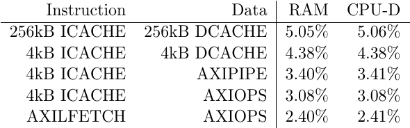Just to prove that this throughput measure isn’t very useful, I found a repeating sequence of 989 clock cycles. In this sequence, there were a set of 41 reads spaced 23 cycles apart, followed by one write beat. This sequence then repeated many times over. Notice how dense such a sequence is, or rather isn’t: one write beat takes place every 989 cycles. Our bus is actually much faster than that. On top of that, the CPU had to do some calculations in the meantime as well, so … the statistic is really quite meaningless.

At another location, I found a set of 5,163 clock cycles for 64 read bursts. After these cycles, the bus was then idle for another 18,846 cycles. This is actually really good performance, since this was from one of the cached tests. The first 64 read bursts filled the appropriate cache lines, and then those lines were used during the next 18,846 clock cycles. The challenge with total throughput here, is which measure would you use? The 2% bus throughput measure, derived from (18846+5163)/64, or the 10% measure derived from 5163/64?

The true answer is neither, since neither statistic really tells us anything about what was taking place on the bus during this time.

In hindsight, if you look back at the throughput measure, the low throughput measure is actually the best indication we have of good cache performance, since a good cache will make it so that the CPU doesn’t need to use the bus at all. Less than 1% throughput, for a cache therefore, is really a good thing.

Perhaps we might have learned more if we had limited our operation to a memcpy() routine, but that’s more of a specialized measurement than what we are looking at today.

Actual Throughput

If we instead limit the throughput measure to the number of beats divided by the number of clock cycles devoted to those beats alone, we’ll get something useful. Before showing the numbers, though, let me remind you that my goal in bus operations has always been 100% throughput. That also means that my AXI block RAM model can achieve 100% throughput in bench testing. How do you think it did in practice?

Here’s the read throughput numbers:

Fig 13. Read throughput (Beats / Cycle)

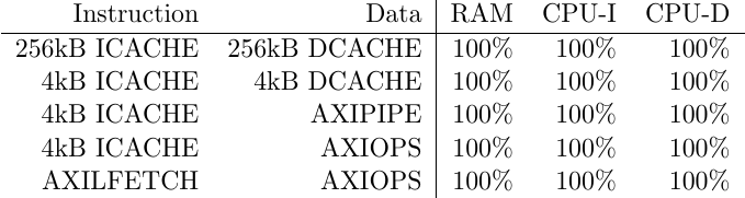Much as I might expect, these numbers are kind of boring. The read throughput statistics above simply show that I’ve achieved the 100% throughput I had intended.

Not very interesting.

What gets more interesting, through, are the write throughput numbers. These were a bit unexpected.

Fig 14. Write throughput (Beats / Cycle)

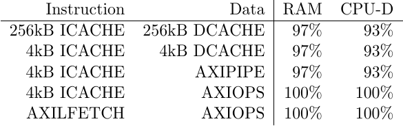I’ll admit, these numbers gave me a bit of a pause. Why shouldn’t I be getting 100% throughput? I had designed this AXI block RAM controller to achieve a 100% throughput, but the measures indicate I was getting something less.

To find out what was going on, I had to do a bit of digging. Fig. 15 below shows what I found: the write channel had stalls and delays within it that I wasn’t expecting.

Fig 15. Write channel alignment stalls limit throughput

If you’ll remember, the RAM can’t perform a write until both data and address are available. To make this happen, I designed the write channel so that it was one cycle delayed from the read channel. As long as the write channel could stay so delayed, we could maintain 100% throughput.

So, let’s walk through the delays in this figure.

The first delay takes place within the interconnect. The interconnect can’t forward any requests downstream until it has first decoded the slave’s address, and then second it has to win arbitration to be granted access to the slave. Unlike the RAM controller, however, the interconnect balances the write address and write data channels during this time. This is the yellow ellipse, shown in Fig. 15 above.

The problem isn’t really the yellow ellipse, it’s the many red ones.

The problem starts because the write address and data from both the CPU and the interconnect is are aligned together, but that’s not good enough for the block RAM controller. The block RAM controller then needs to stall the write data channel by one cycle in order to use it.

This stall then propagates back through the interconnect to the CPU.

In the CPU, however, this creates a bit of an additional problem, since the CPU insists that all memory operations start on a fresh cycle. There’s no buffer inside the CPU for unaligned write address and write data operations. Hence, the last AWVALID is delayed when the CPU cannot issue a new AWVALID && WVALID. This then propagates back down stream into an additional delay on the channel beyond what the block RAM controller required, but as a clear consequence of both it and the fact that the interconnect had no FIFOs within it–only skid buffers.

Put together, we have seven clocks from the CPU used to send five beats of data, for an overall 71% throughput for this burst. Since most of the other CPU writes were for single beats, the total throughput recovers somewhat from this number.

While I might say, thankfully, this only happens about 3% of the time, it’s really not anything to be thankful for. The 3% of the time when this happens just happens to be those few times when the CPU can pipeline its writes so that multiple write operations can be strung together. Typically this happens at the prologue to a function, although it can happen elsewhere. This CPU “feature” is supposed to be associated with better performance. Usually it achieves it, although not this time.

Let’s just say that I’m going to add this to my list of things to fix. The block RAM controller’s performance shouldn’t be causing cascading stalls throughout a larger system.

Latency

Latency, however, is where things start getting really interesting. As you may recall, the read routine requires an extra clock cycle after the read request before it can produce an output. Therefore, we expect a latency of 1.0 from this routine. The interconnect introduces three cycles of latency going in, and an additional one coming back out. So, we might expect read latencies of one and five cycles depending on which side of the interconnect we are on.

Further, if you look at Fig. 16 below, you’ll see that some of the numbers there reflect these predictions. Unfortunately, only some of these numbers reflect these predictions.

Fig 16. Read latency (cycles per burst

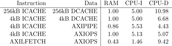What happened?

Let’s look.

First, the measure here that made the least sense to me was the 11 cycle read latency, so I went and dug into that one first.

As it turns out, the 11 cycles were dominated by reads from the console peripheral, as the CPU polled the console peripheral to see if space was available in the transmit queue.

Fig 17. UART transmit FIFO polling latency

In this case, the CPU would issue a request and it would take two cycles to come out of the interconnect. Another cycle was required to bridge the request from AXI to AXI-lite, and then another two cycles to go through the AXI-lite interconnect. Once the request finally got to the peripheral, the peripheral didn’t have a skid buffer attached, so it took another cycle to get through the peripheral. (Why should a UART peripheral need to be fast?) Once the peripheral finished the read, it then took one cycle per layer to get back from there to the CPU.

The fact that the performance was dominated by these peripheral reads is actually a good story, not a bad one. Remember, this measurement is the worst on the data cache test. What that means is that the data cache worked so well, that the cache only needed to issue 12 (burst) read requests of memory. (The instruction cache had to issue more, issuing 50 read requests of memory.) These requests required 5 cycles of latency. However, these five cycles of latency for 12 requests had to then be averaged with another 1,557 cycles of console port polling. Guess which reads dominated the statistic?

But what about the bursts with a latency less than one cycle? This is also another good news story, as shown in Fig. 18 below.

Fig 18. CPU read latency in the presence of singleton reads

In these cases, the controller was issuing multiple reads at a time. Remember, I chose to define latency as the number of latency cycles divided by the number of bursts. Since the number of bursts is higher, the latency is therefore much lower. In the case of Fig. 18 above, you either have 6 beats of latency taking place over 9 burst requests, or 11 cycles of latency divided by 9 requests. Either way you look at it, the latency measure will be less than one.

This should also explain the write latency–from the CPUs perspective.

Fig 19. Write latency (cycles per burst)

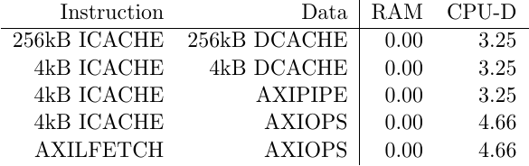The big difference here is that the write latency, from the perspective of the CPU, often includes the interconnect delay–which tends to mask the latency performance of a singleton request somewhat.

But, how did the write latency end up at zero from the RAM’s perspective? The simple answer is that all of the RAM’s write latency was hidden by the write throughput measures, and counted against throughput.

Looking back over read latency measures in Fig. 16, however, shows that I’m not really answering the question I wanted. Because the latency beats are getting averaged by the number of bursts those beats cross, the latency number I’m expecting has been somewhat obscured.

How shall I determine the actual read latency of a given peripheral then?

This was where I came up with the first-request latency measure that I’ve now started using for reads. Although this measure was an after-thought, it seems to capture more of what I’m looking for: the time from the first request to the first response. This measure is shown in Fig. 20 below.

Fig 20. Latency from first read request to first response

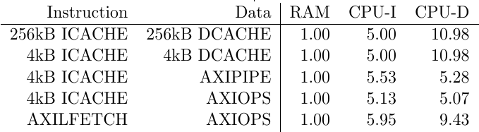Indeed, this is closer to what I was expecting–even though it’s not nearly as useful when predicting CPU performance in this context. First, notice that the block RAM controller’s performance is exactly what I would expect: One clock. The other numbers, however, aren’t quite as clean. This may be due to bus contention between the CPU’s instruction and data buses, but I haven’t dug in deep enough to certain (yet).

Efficiency

While efficiency wasn’t one of my primary measures, I chose to include it in the end because it’s a very simple measure of the bus. Specifically, efficiency as defined below is the number of beats transferred divided by the number of clocks the bus is active. It’s only subtly different from our throughput measures–with the big difference being that the efficiency measure below includes any latency as part of the measure.

Looking at the read efficiency in Fig. 21 below, you can see that the block RAM controller has done fairly well at 80%.

Fig 21. Read efficiency (beats / cycles used)

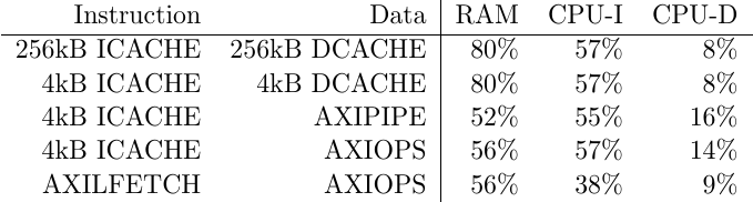This means that the block RAM controller can return 8 beats on average in 10 cycles.

Shouldn’t it be able to do more? Well, yes, it was designed to have a 100% throughput, and we said it had achieved that above. This efficiency number, however, also captures the effects of the interconnect’s single source limitation: both the instruction cache and the data cache only ever issue read requests for eight beats at a time, and the interconnect won’t connect another AXI master to the block RAM controller during this time. Instead, the interconnect waits until the last beat from the CPU instruction master/source has been returned before switching which master is connected to the block RAM controller. This means that, from the RAM’s perspective, each of these cache requests takes two cycles of setup plus another eight cycles of data. This measure captures that performance.

If for this reason alone, the efficiency is a valuable measure.

But what happened with the 8% efficiency of the data cache? Again, this follows from Fig. 17 above. If the data cache is spending it’s bus time polling from a UART with a less than optimized bus response simply because the cache works so well that it doesn’t need to fetch data from the bus, then that’s a good thing. The number just looks bad.

What bout the 38-57% efficiencies shown from the perspective of the CPU instruction fetch interface? Well, if we allow that a cache access requires 10 cycles for 8 beats in the RAM, and we add another 4 cycles for the interconnect, then we have 14 cycles for 8 beats. That’s the 57% efficiency seen. Efficiency, however, gets harder to determine when the CPU keeps deciding, mid-access, that it wants more instructions–such as Fig. 18 showed above. Indeed, this figure alone would explain a 43% efficiency showing that this low-logic approach isn’t nearly as efficient as we might want.

Fig. 22 below shows our calculated write efficiency.

Fig 22. Write efficiency (beats / cycles used)

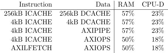To understand these numbers, consider the single write burst shown in Fig. 23 below, in addition to the burst I’ve already presented in Fig. 15 above.

Fig 23. Write efficiency of a single beat

At its most basic, the single write beat of Fig. 23 working its way through the block RAM controller will only ever get a 33% efficiency. From the perspective of the CPU, that efficiency goes down to 14%. The question here isn’t why the write efficiency in the table in Fig. 22 is so low, but rather why is it so good?

The answer to that question let me refer you back to Fig. 15, where in spite of the stalls rippling through the system the RAM controller is still able to support 5 write beats in 7 cycles (71%), and from the CPU data controller’s perspective, 5 write beats in 12 cycles (42%).

The fact that our efficiency is higher than 33% or 14% respectively is due to the CPU’s ability push multiple data beats through the bus pipeline at the same time. Perhaps you may recall this same discussion some time ago with respect to the Wishbone bus and blinky? Pipeline bus operations are definitely the way to go–if you have the area resources to support them. The more operations you can push onto the bus at once, the better your performance will be.

Conclusions

While I don’t expect this to be the last word on AXI performance measurement, the measures presented above have certainly encouraged me to look deeper into how well the bus was working. The process has also helped me understand how well the ZipCPU’s new bus infrastructure worked in a simple setting.

I certainly learned a lot of things in this process.

Some of these lessons learned were to be expected:

1. Raw throughput measures are next to useless. When a CPU is using data and instruction caches, it is a good thing when the CPU is not using the bus. Performance measures shouldn’t penalize such masters for not using the bus.

2. Individual burst performance isn’t necessarily indicative of system performance. As an example, consider the write performance in Fig. 23 and compare it with the write performance of Fig. 15. The correct answer was some combination of the two.

3. There’s a lot of performance lost in the interconnect.

This is a conclusion we came across some time back when examining why a CPU makes blinky run so slow. AXI IDs are supposed to be able to mitigate some of this problem in busy systems, but my own interconnect will need an upgrade to support this feature.

These were the lessons I was expecting to see. There are a bunch of other things I came across during this exercise that I wasn’t expecting.

1. When the cache works well, system performance will be dominated by the slower parts of the system. Yes, I was quite surprised by the exceptionally large read latencies observed when running under the cache. The fact that these latencies were dominated by the printf()’s that run at the end Dhrystone, after the bench mark speed test is complete, was a complete surprise to me.

2. Efficiency, a measure that combines throughput and latency together, is a valuable combined measure. The efficiency measure I came up with was, in many ways, an after thought–yet it seems to be the most concise measure of performance I came up with.

3. My “Perfect AXI slave” block RAM controller isn’t nearly as perfect as I thought it was. Delaying the write data channel certainly has consequences that back up throughout the system. I may therefore need to come back to this “Perfect AXI slave” and adjust it so that it can handle balanced write address and write data channels.

4. Another solution to the problem of the write data and address channels being unbalanced would be placing a couple of FIFOs into my interconnect. So far, I’ve been loathe to do so for several reasons. Chief among these reasons is latency: I’m not sure I want to add to the latency of the entire system by adding another clock (or two) of latency on each channel sufficient to support the FIFO and keep it off of the critical path.

Thankfully, with the performance measures we’ve discussed today, I should now be able to answer the question of whether or not an additional delay improves overall bus performance overall or not.

This leaves me with two pieces of unfinished business. First, the measures we’ve built today are great for a dual port RAM, but perhaps not nearly as good for a single port RAM where the read and write channels need to be joined at some point. The problem is that, from the perspective of a single data channel, the time required to wait for access to the RAM in the desired direction is just counted as stalls. There’s no way to account the two together (currently) to get a combined read measure.

Finally, I’ve been more than tempted to connect this performance monitor to some Vendor components. For example, [FlorentW] wrote an article discussing how to connect a performance monitor to the AXI links within a design using Xilinx’s interconnect and IP integrator. That should lead to a lot of fun measurements, and might finally allow me to measure the performance of their DDR3 controller, whether with or without the PS, or even the performance of their DMA controller against my own.

Indeed, just being able to measure bus performance is really only the first step in a much longer journey. Now I have lots of things to measure the performance of, and so a lot of work still to follow.