Adjusting our logic PLL to handle I&Q

Some time ago, I posted an article on how to create a basic logic PLL in Verilog. The design was simple, basic, and easy to implement in an FPGA. It worked by tracking the most significant bit of any sinewave given to it, giving it a nice gain invariance which would make it useful in a large variety of contexts.

More recently, I was asked to build a demonstration design for a software (gateware) defined radio. Yes, I call it a “software” defined radio, although in actuality all of the processing within it is done by the FPGA. There’s no CPU involved, so perhaps it is better termed as a “gateware” defined radio. I’m going to stick with the “software” label for now–under protest if I have to. Why? Because like a true software defined radio, you really need to know and understand the guts of this one in order to get it to work. Further, as with any FPGA design, this radio design is fully reprogrammable.

The design was to have both AM and FM examples within it. When I went to build those examples, I quickly realized that both the AM demodulator and the FM demodulator would require a PLL that could track the incoming carrier frequency. An ideal candidate for this PLL was my previous logic PLL. The only problem was simply that the logic PLL only worked on a single sinewave input, rather than the quadrature input available on this board.

Today, let’s take a look at why a quadrature demodulator is a good thing, and then look over the difference between the two cores. We can then compare the performance between the two cores so you can see why a quadrature PLL is really a good idea.

What is Quadrature?

The word “quadrature” in today’s article is a reference to a transmit or receive architecture that uses two “arms” or “rails” as they might be called to either transmit, or receive an incoming signal.

Fig 1. A quadrature transmit scheme	Fig 2. A quadrature receiver scheme

Since each arm of a signal in such a scheme is controlled/represented by either a real or an imaginary signal, depending on the arm, I think of “quadrature” signals as a reference more to the complex nature of the signal than to the structure used to create it. In engineering, the two axes of this complex plane are often called “in-phase” or I, referencing the “real” signal rail that is multiplied by the cosine term, and “quadrature” or Q, which references the rail multiplied by the imaginary sine term. The quadrature PLL we are discussing today is one that takes both I and Q inputs.

But let’s back up a bit. There’s a reason why imaginary numbers are imaginary. The square root of negative one can’t really be produced in any physical system, so what reality does this even pretend to represent?

That’s a good question, so let’s start at the top and examine a radio frequency (RF) receiver.

From an engineering standpoint, a good RF front end consists of an antenna, a low-noise pre-amplifier, a band-pass filter, an optional adjustable or automatic gain, an RF mixer followed by a lowpass filter.

Fig 3. A basic RF front end

Mathematically, I like to cheat and just represent a receiver as a downconverter followed by a lowpass filter and then a downsampler.

Fig 4. A simplified receiver model

It just makes the processing easier to understand.

At issue in today’s discussion is the form of the RF mixer, whether the form shown in Fig. 4 above or in Fig 2 above that.

One common way of building a mixer is to simply multiply the incoming signal by a sinewave above or below the signal of interest. This is part of the super-heterodyne receiver architecture. Assuming a signal frequency of f_c and a local oscillator frequency, within the receiver, of f_LO, the resulting signal will be placed at frequencies f_c+f_LO and f_c-f_LO. (We’ll see this in a moment.) A lowpass filter can then be used to select one of these two frequency bands, making it possible to then work on the signal at a lower (and slower) frequency–perhaps even in the digital domain.

Not so with this receiver.

No, the SX1257 Radio PMod uses a quadrature mixer. Within the SX1257, the local oscillator consists of both sine and cosine components. Together, they downconvert a signal much like multiplying by a complex exponential would. The nice part of this setup is that the final signal can be placed near zero frequency–rather than some intermediate frequency offset from zero.

Mathematically, this can really simplify the analysis. There is an engineering cost, however, to making sure that the two “rails” are properly balanced–but that’s not our topic today.

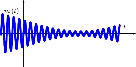
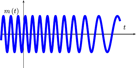
So, imagine if we started with an AM signal. This AM signal is created from some real (not imaginary or complex) information signal, we’ll call it m(t), containing whatever it was we want to transmit and then recover. Inside the transmitter, m(t) will be multiplied by a cosine wave to bring it up to a radio frequency, just as we showed in Fig. 1 above. 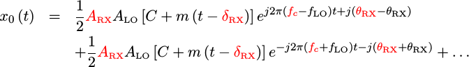After propagation decays and delays this signal and noise gets added to it, it might then show up to the receiver looking something like:

where

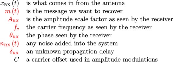Our goal will be to recover the message, m(t).

You may have noticed the colors in the expression above. I like to do this to help me understand what it is I have to work with. In particular, I like to write out all of my unknown values in red. In general, the whole expression is red save for the waveform we’ve measured. We can argue about whether or not the amount of carrier, C, is known or not–in the end it’s not all that relevant since we’re just going to filter it out anyway.

Several of these terms take a lot of work to track from the origin to the receiver. Particularly complex terms include the amplitude, A, the propagation delay, delta, and the phase. Each of these is related to how the waveform propagated from the source to the receiver, so they cannot necessarily be known when the waveform is received. Worse, they are particularly difficult to track and apply meaning to even in the receiver since so many components of the receiver’s processing path adjust them along the way.

For example, our first step in processing this signal will be to adjust the frequency to “baseband”–where the frequency of the cosine term gets (approximately) zeroed out. Let’s suppose we know about what fc is so that we can create a local oscillator (one generated in the receiver) at something close to f_c–let’s call it f_LO for the frequency of the local oscillator. We might then multiply x(t) by this local oscillator to get a baseband signal.

If we ignore the noise term for now, we can expand this out a bit to simplify it.

If we then use a lowpass filter to remove the term at f_c+f_LO, we can then get a useful waveform to work with.

Did you notice how the amplitude, frequency, and phase all changed during this process? Keeping track of all of these changes can be quite a challenge. It’s often much easier just to merge the details of the local oscillator processing stage together with the values of the signal that are already unknown. Therefore, I will often create new frequency and phase terms just to keep my notation simpler.

This newer, simpler, signal description is still the same thing that we were just looking at.

AM Demodulation

Let’s pause for a moment and consider what this m(t) signal might “look” like.

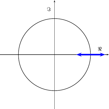
First, we know that m(t) was real.

Fig 5. Initial message signal in time

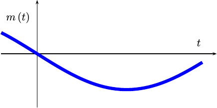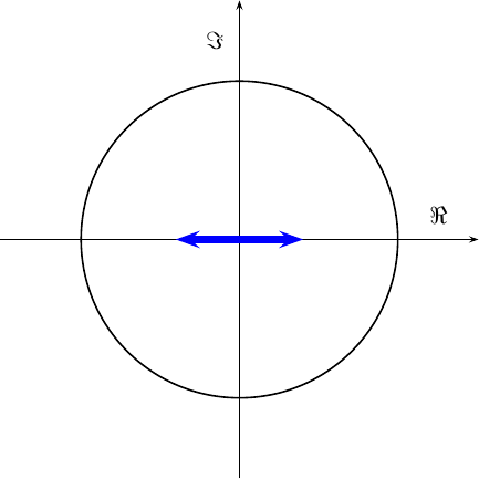
If we place rotate this figure so that time goes in and out of the page (screen), m(t) can then be plotted on a complex plane and it would look like points along the x axis as shown in Fig. 6 below.

Fig 6. The initial message shown as a phasor

If we then add the AM carrier offset C to it, the message points just shift to the right.

Fig 7. The initial message, but offset by the constant carrier

Once the message gets multiplied by a complex carrier, this diagram starts spinning in circles at the carrier frequency.

Fig 8. The transmitted waveform, spinning at RF frequency

Of course, only the real component of this diagram will ever get transmitted, so the picture over the airwaves will likely look like a more traditional AM signal.

Fig 9. The transmitted waveform, as viewed in time

Inside our receiver, we’re going to try to de-spin this signal. If we do the task right, so that f_c == f_LO, the incoming signal will look something like,

Fig 10. The received waveform, once the carrier has been removed

At this point, we don’t want just the real or imaginary portions. Were we to only grab the real component, as an example, there would be a worst case where we might just happen to get so unlucky that we lose the entire signal.

Fig 11. The received waveform, once the carrier has been removed

We could’ve picked some intermediate frequency, f_IF such that f_LO = f_c - f_IF. Had we done that, our signal would’ve still been spinning as it was in Fig. 8 above, just spinning slower. We’d still need to eventually remove the rotation, so we’re going to get to Fig. 10 either way.

If f_LO is only approximately equal to f_c, such as would be the case in real life, then this constellation plot would rotate slower. Our goal, as part of our AM demodulator, is going to be slowing and eventually stopping this rotation. We’ll then want to rotate the constellation that results back to zero phase, and to remove the carrier offset.

Tracking this rotation is the purpose of our quadrature PLL.

FM Demodulation

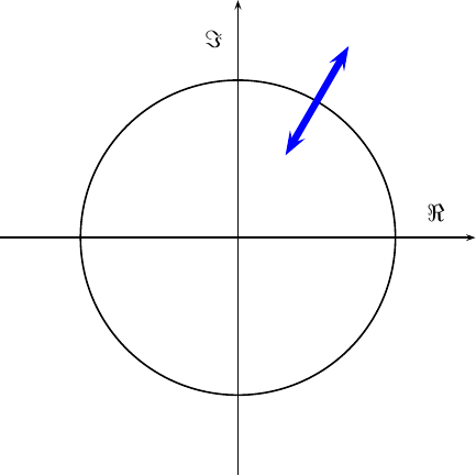
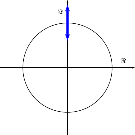
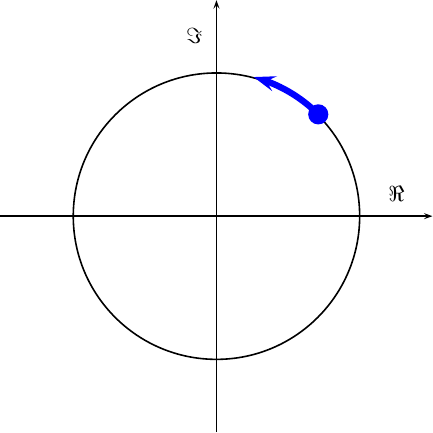
If we were to start with frequency modulation (FM), the signal might not necessarily be real, but many of the same principles would still apply. In this case, the signal would start out slowly rotating back and forth around the complex plane.

If the frequency excursions were small enough, they could be approximated as purely imaginary excursions from the right side of the unit circle, as shown in Fig. 12 below.

Fig 12. A narrowband FM signal

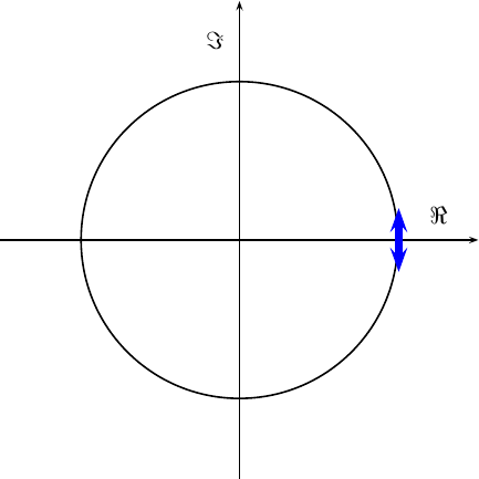If they are larger, the approximation no longer applies, but it’s still FM.

Fig 13. A widerband FM signal

How big the frequency changes within the message are is a function of how the system is set up.

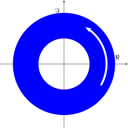
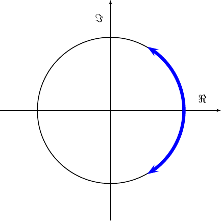
As before, the transmitter spins this signal.

Fig 14. The transmitted waveform, spinning at RF frequency

Unlike the AM signal shown in Fig. 8, this signal has a constant amplitude, as shown by the narrow line drawing the blue circle in Fig. 14. The transmitter then transmits only the real portion of it,

Fig 15. The FM waveform, as transmitted, but shown in time

because imaginary signals are only imaginary–right?

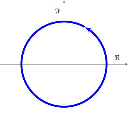
Inside the receiver, our goal will be to first remove most of the spinning, and then to capture the spin frequency as our resulting message.

As with the AM demodulator, the FM demodulator, can be accomplished with a PLL. Likewise, the quadrature information helps to keep us from diabolical cases. In the end, our task is essentially to measure the speed of a point as it spins around a circle in the complex plane.

Fig 16. Demodulating FM is about determining the speed of rotation about the circle

Adjusting the Phase Detector

When we first built our PLL, we had to do a lot of work to figure out whether or not the PLL phase was ahead of or behind the incoming sinusoid. This required finding when the two inputs agreed with each other, and then looking at which input changed first to know which of the two clocks was faster or slower.

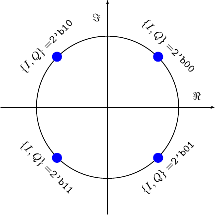
With quadrature signals, things are different. The first change will be admitting two input bits, one for I and one for Q, into our core.

	input	wire	[1:0]		i_input; // = { I, Q }

These two incoming bits can be used to approximate the incoming phase as either 45, 135, -135 or -45 degrees.

Fig 17. Incoming IQ phase map

Similarly, the top two MSB of the phase counter internal to our PLL can also be mapped to these same points.

Fig 18. Phase as given by the top two MSB bits of the phase counter

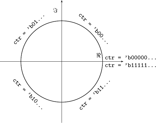The mapping isn’t quite the same, so we’ll need to watch out for this difference as we go along.

Our next goal is to determine whether or not a phase error exists. Are these two waveforms locked, or should we adjust the phase within our PLL?

	always @(*)
	case({ i_input, ctr[MSB:MSB-1] })
	4'b0000: phase_err = 1'b0;	// No err
	4'b1001: phase_err = 1'b0;	// No Err
	4'b1110: phase_err = 1'b0;	// No err
	4'b0111: phase_err = 1'b0;	// No err
	default: phase_err = 1'b1;
	endcase

Notice how the two coordinate systems, that of the I,Q input and the phase counter, are not the same. You can use the figures above to help decode them. (While it felt like I was counting on my fingers, I got so confused I had to use similar figures to work out which quadrants of each represented an error and which did not.)

I also wanted a second bit as well–one that wound indicate whether or not the PLL’s frequency should be increased or decreased. A decrease in phase (and frequency) would be warranted if the PLL’s counter was ever further clockwise than the incoming phasor, otherwise an increase of each would be appropriate.

Fig 19. Lead vs Lag

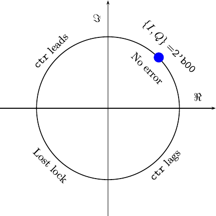But what if the two are in opposite quadrants? That is, what if the I,Q input represents a 180 degree difference from the angle represented by the PLL’s counter? In this case, I chose to go both ways–for two quadrants I judged the phase to be too far forward, and for the other too far backwards. The resulting table, including the phase error from above, is shown below. It should match Fig. 19 for the first quadrant, and similarly for the other three.

	//
	// Input {I,Q} (i.e. X,Y) will rotate: 00, 10, 11, 01
	// The counter will rotate: 00, 01, 10, 11
	//
	always @(*)
	case({ i_input, ctr[MSB:MSB-1] })
	//
	4'b0000: { lead, phase_err } = 2'b00;	// No err
	4'b0001: { lead, phase_err } = 2'b11;
	4'b0010: { lead, phase_err } = 2'b11;
	4'b0011: { lead, phase_err } = 2'b01;
	//
	4'b1000: { lead, phase_err } = 2'b01;
	4'b1001: { lead, phase_err } = 2'b00;	// No Err
	4'b1010: { lead, phase_err } = 2'b11;
	4'b1011: { lead, phase_err } = 2'b01;
	//
	4'b1100: { lead, phase_err } = 2'b11;
	4'b1101: { lead, phase_err } = 2'b01;
	4'b1110: { lead, phase_err } = 2'b00;	// No err
	4'b1111: { lead, phase_err } = 2'b11;
	//
	4'b0100: { lead, phase_err } = 2'b11;
	4'b0101: { lead, phase_err } = 2'b01;
	4'b0110: { lead, phase_err } = 2'b01;
	4'b0111: { lead, phase_err } = 2'b00;	// No err
	endcase

The fun part of this table is that despite its ugly form, it can be implemented with nothing more than two 4-LUTs.

But what about that 180-degree out of phase measurement? You could think about it as an annoying offset to figure out lead and lag for, or you could look at it as an opportunity. If the phase measurement is ever so far out of phase that we can’t tell which came first, then we are clearly out of lock.

We can use this to generate a crude lock indication.

module	quadpll(/* ... */ o_locked);
	// ...
	output	reg			o_locked;

We can set this lock indicator to be low any time we are off by 180 degrees, and high otherwise. True, it’s crude. Any phase errors between -135 and 135 degrees will appear to be locked. Worse, this lock indicator will appear to glitch if it ever falls out of lock. However, such glitches should be easy to quickly identify on a trace, and so use to know if the PLL is properly locked or not.

	always @(posedge i_clk)
	if (i_ce)
	begin
		case({ i_input, ctr[MSB:MSB-1] })
		//
		4'b0010: o_locked <= 1'b0;
		4'b1011: o_locked <= 1'b0;
		4'b1100: o_locked <= 1'b0;
		4'b0101: o_locked <= 1'b0;
		default: o_locked <= 1'b1;	// Everything else
		endcase
	end

The rest of the design, to include how we tracked both phase and frequency, is the same as our prior design. That means our tracking loops should all have the same gains and transfer functions. In other words, they should perform the same … right?

Let’s take a peek.

Performance difference

The good news with this new quadrature PLL implementation is that it is so similar to our last one that we can nearly use the same Verilator script. Indeed, a graphical diff, shown in Fig. 20, shows how similar the two scripts actually are.

Fig 20. Test script differences

The biggest difference between the two scripts is how the phase is sent to the core. In our original test script, we defined the phase going into the PLL as nothing more than the MSB of the phase counter.

                lclphase += lclstep;
                tb.i_input = (lclphase >> 31)&1;

It’s a little more involved for the quadrature PLL, since we need to convert from the coordinates of the top two counter bits, as shown in Fig. 18 above, to the IQ coordinates used by the core, as shown in Fig. 17 above.

                lclphase += lclstep;
                tb.i_input = (lclphase >> 30)&3;
                // 00 10 11 01
                switch(tb.i_input) {
                case 0: tb.i_input = 0; break;
                case 1: tb.i_input = 2; break;
                case 2: tb.i_input = 3; break;
                case 3: tb.i_input = 1; break;
                }

I say a “little more” involved, because this really isn’t that big of a change.

Surely this wouldn’t affect performance, right?

Well, let’s take a look at the phase error outputs and compare the two over time in Fig. 21.

Fig 21. Absolute phase errors

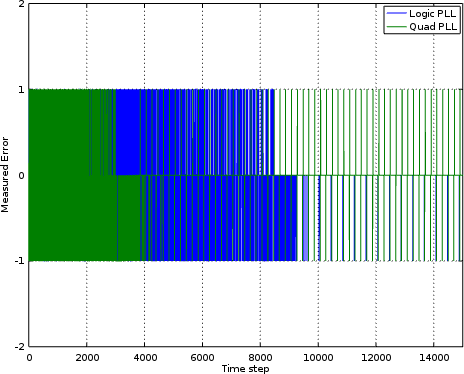In this chart, the error is a -1 if the PLL is leading the incoming signal, 1 if the PLL is lagging behind and 0 if the two match. Unfortunately, this 2-bit error quantization approach hasn’t left this chart very readable. Still, we might stare at Fig. 21 long enough to imagine that after about 4k samples the quadrature PLL no longer had the error the logic PLL was struggling with.

But are we only imagining this?

Well, I suppose we could cheat and examine the various phase counters from within the PLLs and compare them to the original counter used to generate the signal itself. If you do that, you’ll get something that looks like Fig. 22.

Fig 22. Instantaneous phase counter error

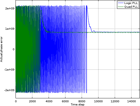As with the previous figure, there’s a lot of junky noise on the left side of this chart. This is due to frequency error, and marked by the phase wrapping around the unit circle and back again. The large units, +/- 2e9, are simply the units of the phase counter that we are using. Even in this figure, however, it appears as though the quadrature PLL’s phase error converges on a right answer much faster than the logic PLL’s error does.

Is there a way to “see” though this junk, though, and get a better picture of what’s going on?

To find out, let’s average our phase error and see which one gets closer. Using the same boxcar filter applied to the phase error output from both PLL’s, we see an averaged phase error plotted in Fig. 23 on the right.

Fig 23. Averaged phase errors

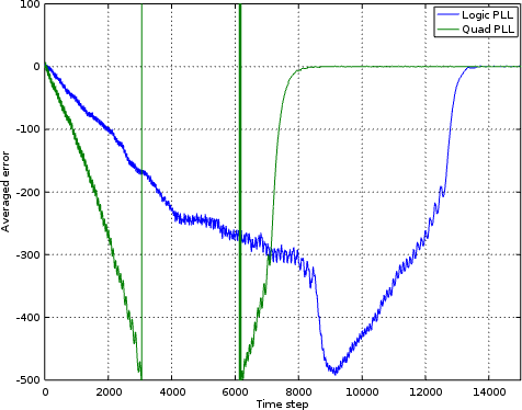In this chart, it appears as though the quadrature PLL quickly ran up a phase error so large it wrapped around the unit circle. The quadrature PLL then went from estimating a lead to estimating a lag. However, before you draw too much of a conclusion from that, you need to notice that it recovers very quickly and that from a point of about 8k steps on there’s essentially no averaged phase error in the quadrature PLL whereas the logic PLL we built earlier still takes another 5k samples or so to lock.

Are we really achieving a faster lock?

Let’s peek inside the two cores and check their frequency steps. As you may recall, the frequency “step” is really a phase step that’s used to implement a frequency. As with our other phase units, this step ranges from -2e9 to 2e9, although the chosen “correct” answer is found somewhere near 8.25e8. Both PLLs are started with the same erroneous frequency, and then tasked with finding and tracking the right one. Fig. 24 shows the frequency steps of the two PLLs as they each attempt to track the frequency of the incoming waveform.

Fig 24. Frequency step vs time, showing frequency acquisition time

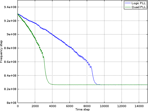By this time, the result comes as no surprise. The quadrature PLL indeed acquires a phase lock much faster than the basic logic PLL.

Perhaps this shouldn’t come as such a surprise. While both cores are using the same tracking loop, the quadrature PLL has a better phase estimator. Better information going into the loop should result in better performance, which is what we’ve seen in these figures. As far as whether the performance is really 2x better, I’ll let the charts speak for themselves.

Conclusions

With only a few minor modifications, we were able to transform our simple, basic logic PLL into a full-blown quadrature PLL for software (gateware) defined radio applications.

How well does the new PLL work? Judging from performance simulations, it works much better than the prior PLL. How about in actual practice? Sadly, I have yet to put the two radios together on my desk to measure how well either the AM demodulator or the FM demodulator actually performs. Until then, I suppose these simulations will feel real good while never quite being the same as the real thing.

As it is, I’ve already got another discussion queued up regarding how I built the downsampling filters for the two demodulators. Those should form another good discussion, since it’s an important part of digital filtering that we have yet to discuss on this blog.