Building a Numerically Controlled Oscillator

Many signal processing applications require a sine wave at some point. If the phase or frequency of this sine wave is controlled within the design, then it is often called a Numerically Controlled Oscillator (NCO). Let’s spend some time today looking into how you might build one of these within an FPGA. We’ll also present a C++ implementation at the end as well, which may be used in embedded applications.

Since we’ve already studied how to generate a sine wave on an FPGA, most of our work is already done: We’ve discussed a table lookup method, a quarter wave table lookup, method, and even how to generate both a sine wave and a cosine wave using a CORDIC. The subtle difference to describe to day is really how to turn such a sine wave generator into a NCO.

Before we dive into the details, though, let’s spend a moment thinking about how you might use such an NCO. My own reason for presenting this today is twofold. First, I know of a student struggling to understand how to build something like this as part of a digital communications demodulator. There is a small trick involved–one that appears to be well known among those who do this sort of thing for a living, but not so well known among students and I’d like to share it here. Indeed, I think we might even build a better NCO below than this stackoverflow article recommends. My second reason for writing today is that I’d like to write about how to build a Phase Locked Loop (PLL) within an FPGA on this blog, and every PLL I’ve ever built has always included the basic NCO logic as part of its implementation.

But this hardly scratches the surface of what you might do with an NCO. Consider as an example that …

Any linear signal processing system is completely characterized by its frequency response. As a result, I’ve used an NCO in time past, together with a scope of some type, to evaluate whether the digital input to a signal processing algorithm was being handled properly.
We used an NCO earlier as part of our demonstration that the improved PWM generator worked better than a traditional PWM for audio signal generation. While we didn’t discuss the details of the tone generator at the time, we’ll explain many of those details today.
You can also use an NCO to move a signal around in frequency–either bringing it down from some intermediate frequency (IF) to a baseband frequency where you can process it in a receiver, or the same in the other direction as part of a transmission algorithm.
You can also use an NCO as part of either a digital communications modulator or demodulator.
You can use an NCO to create an Amplitude Modulated (AM) signal, or even a Frequency Modulated (FM) signal.
Another common use is to generate musical notes via an additive synthesizer. Indeed, the phase accumulator portion of the NCO we’ll develop below can even be used in subtractive synthesis–it’s quite generic.
Finally, because you as the designer have complete control over the frequency output of the NCO, you can even do some more exotic things–such as building a frequency hopping spread spectrum signal–should this be what you wish to do.

Indeed, NCOs are such fundamental components of Digital Signal Processing (DSP) algorithms that it is difficult to enumerate all the things they can be used for here.

What is an NCO?

Fig 1. NCO

For our purpose today, a Numerically Controlled Oscillator is simply an oscillator created from digital logic that you have complete control over digitally. Nominally, such an oscillator will receive as an input the frequency you wish to produce and it will produce a digitally sampled sine wave at that frequency. Should you choose to use an NCO within a PLL, then you will also be adjusting the phase of this sine wave generator. For now, however, consider an NCO to be a simple digital logic circuit that takes a frequency input and produces a sampled sine wave as an output.

Fig 2. Block Diagram

Internally, the NCO keeps track of the phase of the sine wave it produces, and it increments this phase at each sample point.

Let’s walk through a little bit of trigonometry, to see how this works.

We’ll start with the sine wave that we want to produce, such as the sine wave shown in Fig 3,

Fig 3. A pure sinewave

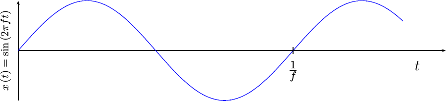and is given by the equation,

Since digital implementations can only work on sampled signals, we’ll need to sample this sine wave every Ts seconds. To keep our notation straight, we’ll now index this sine wave output by sample number, n, rather than by time, t.

I personally find it easier to work with the sample rate of the digitizer, fs rather than the time between samples, Ts. These are reciprocals of each other, so fs = 1/Ts. We can then express this same equation as,

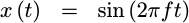
and plot the sampled function in Fig 4.

Fig 4. A sampled sinewave

In this figure, the samples are shown in circles. They are each separated by a phase of 2pi f/fs.

Our entire focus in this algorithm, though, is going to be on the phase of this expression–the argument of the sine wave. In the expression above, this phase is given by n times the frequency ratio, f/fs, times 2pi. We’ll call this changing phase value phi[n].

To build an NCO, we are going to need to transform this phase value, phi[n], into an input our sine wave generator can handle.

We’ll start by rewriting our sine wave using this phase value, phi[n], so that it captures the internals of this sine wave–with the exception of the 2pi portion.

Specifically, this phase value is defined by,

Fig 5. Unit circle rotations

It represents the number of times our sine wave has gone around the unit circle–the number of rotations if you will. For example, a phi[n] of 1.0, applied internally to our sine wave, would lead to a phase argument to our sine function of 2pi–suggesting we had gone around the unit circle once. A phi[n] of 2.0 would yield the same value, but represent instead that the phase had traveled around the unit circle twice. Fractions then will indicate partial angles from the x-axis around the unit circle, hence a phi[n] of 0.5 would represent going halfway round this circle, while 0.25 would represent a quarter of the way around the circle.

Let’s keep working with this value for a bit. We can define this phase recursively based upon the prior phase.

This simple modification accomplishes two purposes. First, it allows us to avoid a multiply by n, turning the calculation of the next phase from the past phase into an operation requiring an addition alone. Second, because this newer version is no longer tied to the distance from n=0, this subtle change allows us to maintain any accumulated phase offsets in our NCO as well–not just frequencies with zero phase at zero time.

This sounds fairly straight-forward so far. What’s the trick?

The “Trick” to building an NCO

The “trick” in building an NCO lies in the units of phi[n]. The units of phi[n], presented above, are a number of cycles (or rotations) around the unit circle. As a result, a phi[n] of 1.0 represents once around the unit circle, and a phi[n] of 2.0 represents twice around the unit circle, etc.

However, within most signal processing logic (not quite all), you don’t care how many integer times a sine wave goes around the unit circle, you only care about the angular fraction. Let’s therefore examine this number in terms of both it’s integer and fractional portions.

Specifically, let’s separate it into an integer portion, and the first W bits past the decimal point as shown below.

$phi[n] separates into integer components and W fractional components$

Pictorially, dropping the integer portion might look like Fig 6 below.

Fig 6. Phase function

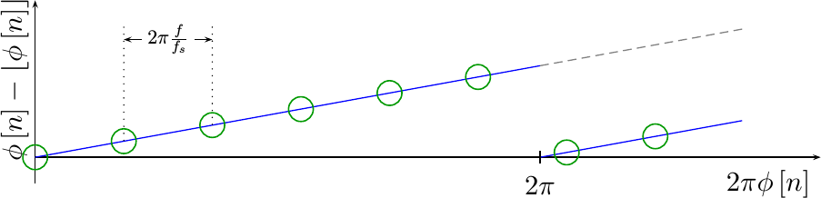Notice how the phase jumps back to zero in Fig 6 at the same point as where the sine wave starts to repeat. Sure, you didn’t need to bring this value back down to zero, but doing so creates a limited range in y that we can then split among a fixed number of bits, W.

Since we didn’t care about the integer number of times we’ve gone around the unit circle, we can subtract from phi[n] its integer portion to recover the fraction alone–just like we did in Fig 6 above. We can then multiply the result by 2^W, so as to get a fixed-point phase representation that will fit within a word of W bits long.

Just to finish this off, we’ll only keep the integer portion of this value, representing the top W bits of our fractional phase, and we’ll ignore any further bits beyond the decimal point.

Hence PHI[n] is now a number between 0 and 2^W-1 representing a fractional rotation around the unit circle, a value between 0 and 1.

That’s the first part of our “trick.”

For the second part of this “trick”, let’s use the top P bits of our phase, PHI[n], as the input to our sine wave generator, whether a table lookup sine wave generator, or even the phase input phase value of a CORDIC algorithm.

But what about the rest of the W bits of our fixed-point phase representation?

These can be used for one of two purposes. First, they can be used as a fractional table index, accumulating over time to adjust our table index. An example of this is shown below in Fig 7.

Fig 7. Fractional phase accumulation
$phi[n] separates into integer components and W fractional components$

If you look carefully at this figure, you can see how the phase pointer moves a little bit more than one table position at a time. Eventually this extra accumulated fraction causes the table index to skip a table position entirely (position 6).

This will allow you to represent and create sine waves at frequencies not formed by integer steps through your table. Such frequencies may involve jumping across table entries, as shown above in Fig 7, or even repeating entries if necessary. Yes, jumping entries will likely cause a distortion in your output, but it will also help you maintain better frequency resolution than the first P bits alone would allow.

A second use for the bottom W-P bits would be as part of an interpolation scheme to reduce the phase noise associated with any table representation. This is such an important possibility that we may have to come back to it and write about it more in a later article.

But, what about overflow?

This is an important question, so let’s walk through an example and see what happens. Consider what would happen if we were keeping track of phase in an 8-bit word, and one of our additions overflowed. For example, suppose you wanted to take four steps to go around a circle, starting at PHI[n]=8'h20 (45 degrees). You’d then add to it 8'h40 (90 degrees) on each clock. The resulting sequence would then be, 8'h20 (45 degrees), 8'h60 (135 degrees), 8'ha0 (225 degrees), 8'he0 (315 degrees), 8'h20 (45 degrees).

Did you catch what just happened? The phase accumulator just overflowed between 315 degrees and 45 degrees, and yet the phase representation just “did the right thing”! What that means is that you can ignore any overflow in your phase–it’s just going to wrap around the unit circle anyway, and the sine wave generator is only interested in the phase fraction anyway.

Example Source Code

So, how would this look in practice? Let’s look at an example of what this would look like in both C++ and Verilog.

We’ll start with a C++ example. We’ll make a C++ NCO class incorporating these principles. There are three basic parts to this class. The first is the class declaration and table generation.

class NCO {
public:
	unsigned	m_lglen, m_len, m_mask, m_phase, m_dphase;
	float		*m_table;

	NCO(const int lgtblsize) {
		// We'll use a table 2^(lgtblize) in length.  This is
		// non-negotiable, as the rest of this algorithm depends upon
		// this property.
		m_lglen = lgtblsize;
		m_len = (1<<lgtblsize);

		// m_mask is 1 for any bit used in the index, zero otherwise
		m_mask = m_len - 1;

We’ll build the table itself with the sine wave values at the left-edge of any interval. This isn’t optimal, since it will force the error to zero on the left edge and likely make it a maximum on the right side of the interval, but it will yield us a decent capability quickly.

		m_table = new float[m_len];
		for(k=0; k<m_len; k++)
			m_table[k] = sin(2.*M_PI*k / (double)m_len);

We may come back to this in a later post to minimize the maximum error in this lookup.

The last part of this initialization is to provide initial values for our phase accumulator (PHI[n]) and the phase step necessary to create a known frequency output. In this case, we’ll initialize this step so that it will produce a zero frequency–not very exciting, but fixing that will be our next step.

		// m_phase is the variable holding our PHI[n] function from
		// above.
		// We'll initialize our initial phase and frequency to zero
		m_phase = 0;
		m_dphase = 0;
	}

	// On any object deletion, make sure we delete the table as well
	~NCO(void) {
		delete[] m_table;
	}

The second part of this implementation is the function that sets the frequency. This is captured within the NCO object by the phase step, m_dphase. As discussed above, this is the difference between PHI[n] and PHI[n-1]. Further, if you create a SAMPLE_RATE value in Hertz, then f can be given to this routine in Hertz. Otherwise, you can keep SAMPLE_RATE set to 1.0 and then the f value accepted by this routine will be set in terms of a normalized frequency ranging from 0.0 to the Nyquist frequency, 0.5.

	// Adjust the sample rate for your implementation as necessary
	const	float	SAMPLE_RATE= 1.0;
	const	float	ONE_ROTATION= 2.0 * (1u << (sizeof(unsigned)*8-1));

	float	frequency(float f) {
		// Convert the frequency to a fractional difference in phase
		m_dphase = (int)(f * ONE_ROTATION / SAMPLE_RATE);
	}

As a matter of personal practice, I never make the SAMPLE_RATE a part of my NCO implementations. That way one NCO implementation can work across multiple projects.

You may find that the most confusing part of the logic above is the ONE_ROTATION value. This is the phase value representing once around the unit circle. It is given by 2^W. We have to go through a bit of a hoop to set this value, though, since the ONE_ROTATION value doesn’t fit within the unsigned integer we are using to hold PHI[n] (m_phase). Alternatively, we might’ve set ONE_ROTATION to pow(2,sizeof(unsigned)*8), but the approach above makes it easier for the compiler to recognize that this value is a constant, rather than needing to call the pos() math library function.

The final part of this class steps the index into the table forward by one step, and then returns the value of the table at the index given by the top P bits in the m_phase word.

	float operator ()(void) {
		unsigned index;

		// Increment the phase by an amount dictated by our frequency
		// m_phase was our PHI[n] value above
		m_phase += m_dphase; // PHI[n] = PHI[n-1] + (2^32 * f/fs)

		// Grab the top m_lglen bits of this phase word
		index = m_phase >> (sizeof(unsigned)*8)-m_lglen);

		// Insist that this index be found within 0... (m_len-1)
		index &= m_mask;

		// Finally return the table lookup value
		return m_table[index];
	}

You may notice that I’ve chosen to use single precision floats, rather than double precision floating point numbers. I did this for two reasons.

First, I wanted to encourage you to ask the question of just how much precision do you actually need?

Second, I wanted to point out that the single precision float representation only has a 24-bit mantissa. Most CPUs today allow integers of 32-bits. As a result, the integer phase accumulator has more precision than a float phase accumulator. You can see this pictorially in Fig 8.

Fig 8. Floating vs Fixed point phase

If you are not familiar with single precision IEEE floats, the first bit, S, is a sign bit, and the next seven, E, are exponent bits. The final 24-bits, M, are mantissa bits. Put together, these items represent a number sort of like, (-1)^S * 2^E * M. (Yes, I’m skipping some details here.)

Unlike IEEE floats, our fixed point phase representation is simply 32 mantissa bits, having a value ranging from 0 to 1.

Which one do you think will have more precision?

In a similar fashion, if you were to use an unsigned long for your accumulator instead of an unsigned value, then the phase accumulator would have more precision than a double precision float would allow.

In both cases the reason why this phase accumulator out-performs a floating point phase accumulator is simple because our representation has a fixed decimal location, rather than a floating decimal point. That allows more bits per word to be allocated to the mantissa, since the floating point representation needed to allocate extra bits for both a sign bit and the exponent.

Were you to build an NCO implementation within Verilog, the code is almost identical. The biggest differences are first the fact that we require the frequency given to be already be converted into the appropriate units, and second that the bit select is simpler than before.

module	nco(i_clk, i_ld, i_dphase, o_val);
	parameter	LGTBL = 9, // Log, base two, of the table size
			W = 32, // Word-size
			OW = 8; // Output width
	localparam	P = LGTBL;
	//
	input	wire		i_clk;
	//
	input	wire		i_ld;
	input	wire	[W-1:0]	i_dphase;
	//
	input	wire		i_ce
	output	wire [OW-1:0]	o_val;

Any time a new frequency is requested, the i_ld signal will be set high and the new frequency placed into i_dphase. This frequency value is in the units of m_dphase in the C++ code above.

	reg	[W-1:0]	r_step;

	initial	r_step = 0;
	always @(posedge i_clk)
	if (i_ld)
		r_step <= i_dphase; // = 2^W * f/fs

Likewise, on any clock where i_ce is high, we’ll step the phase forward by this same frequency-dependent amount.

	reg	[W-1:0]	r_phase;

	initial	r_phase = 0;
	always @(posedge i_clk)
	if (i_ce)
		// PHI[n] = PHI[n-1] + 2^W * f / fs
		r_phase <= r_phase + r_step;

Finally, the top P bits of r_phase are used in our table lookup.

	sintable // #(.PW(P), .OW(OW))
		stbl(i_clk, 1'b0, i_ce, 1'b0, r_phase[(W-1):(W-P)],
		o_val, ignored);
endmodule

You may notice that both the C++ and Verilog implementations are quite similar. They are both low logic implementations showing the basics of what is required to create an NCO.

Future Posts

We’ve just presented the logic behind building a basic NCO. While the sine wave generated by this approach isn’t perfect, it may well be good enough for your project. Should you need a higher quality sine wave, you may wish to know that there are other/better sine wave generators out there beyond the simple table lookup method we’ve discussed before.

As one example of doing better, you may wish to note that we’ve done nothing to minimize the maximum error for any given table index.

In a similar manner, we’ve done nothing with the rest of the W-P fractional bits in our W bit phase accumulator. These bits can be used to interpolate between table entries, either linearly, quadratically, or more as desired for better performance.

These, however, will need to be left for discussions on some other day.