
A Basic Upsampling Linear Interpolator
Our last post on interpolation discussed how to change the data rate of a signal within a system from one rate to another by using a sample and hold interpolator. If you’ve spent much time working with Digital Signal Processing (DSP) algorithms, you’ll understand that this approach offers absolutely no antialiasing protection. Sure, it works, but it’s not necessarily how you will want to build a quality system.
As an example, let’s consider a simple waveform, drawn below in blue.
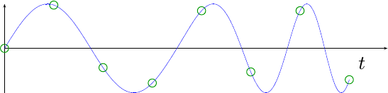 |
This waveform has been sampled at the green dot locations.
If we now used the sample and hold algorithm to resample this signal, we’d get a result looking like the red dots in Fig 2.
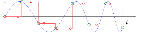 |
While we could center the diagram, and thereby do a nearest neighbour interpolation (Fig 3),
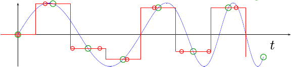 |
the result just doesn’t look much better. It still doesn’t look anything like our original signal, shown in blue.
For this post, let’s try to do one better. Let’s build a upsampling interpolator, that will linearly interpolate between two data points.
What is a Linear Interpolator
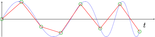
Linear interpolators are very similar to the child’s “dot-to-dot” method of drawing, where a picture is given with numbered dots, and the child must draw a line from one dot to the next. The resulting waveform might look very much like Fig 2 below.
 |
If we now sample this waveform, using an upsampler, we should get the black dots shown in Fig 5.
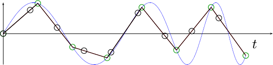 |
Or, if you have a higher oversampling rate (i.e. more green dots), it might look like Fig 3 below:
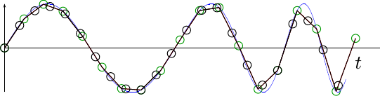 |
At this point, you can see how our sampler starts to track the incoming signal a lot better.
The equation for a linear upsampler, one that generates a line between two given sample points, is straightforward:
n = floor(t/Ts);
y(t/Ts) = x[n] + (t/Ts-n)(x[n+1]-x[n]);
where samples are spaced by Ts seconds apart.
To get a feel for this equation, consider what happens when t=nTs. In
that case, the linear term drops to zero and the result is x[n]. On the
other hand, if t is infinitesimally less than t=(n+1)Ts, then t/Ts-n
will evaluate to 1 and y(t/Ts) will evaluate the x[n+1]. In other
words, this equation simply describes a series of line segments connecting
x[n] to x[n+1].
The linear sampler we are going to build today will return the values
y(kV/Ts), for some new sample interval V < Ts, just likes Figs 5 and 6 above
demonstrate.
This leaves us with two challenges: The first is evaluating the equation for
upsampling, and the second problem is figuring how how to do this evaluation
every V seconds to produce an output.
Handling the incoming clock
The first step towards building this interpolator is to calculate n and
(k (V/Ts)-n). Well, not quite. Practically, there is no need to know
n itself. Indeed, without an absolute time to reference everything to,
n is quite arbitrary. That leaves k (V/Ts) -n. Let’s call this number
dt to facilitate our discussion.
dt is a number whose value goes from zero to one, and then suddenly back
to zero again.
In other words, we can keep track of this number in a similar manner to the
way we kept track of the phase of a sine
wave earlier. To
do this, we’ll keep track of a number between 0 and 2^N-1, which is given by
2^N dt.
To this number, on each clock, we’ll add 2^N(V/Ts) to it (rounded to the
nearest integer, of course). Then, when this
number overflows N bits, we’ll wait for the next sample (i.e. for floor(t)
to go from n to n+1, before using the new phase.
Let’s define a register, i_counter, to hold the integer portion of this
number, 2^N dt. You can make N as big as you need to in order to make
this work. Likewise, we’ll define i_step to hold the delta 2^N(V/Ts).
i_step = 2^N (int)(V/Ts)Now, with these two values, we can calculate the offset from the top of the last sample:
always @(posedge i_clk)
	pre_ce <= i_ce;

always @(posedge i_clk)
	if (i_ce)
		// r_ovfl will get set on any overflow
		{ r_ovfl, r_counter } <= r_counter + i_step;
	else if (!r_ovfl)
		{ r_ovfl, r_counter } <= r_counter + i_step;
Notice how, when any new sample arrives, we update our counter (and produce an output). Likewise, until the update overflows, we’ll keep updating the counter and producing an output.
This sounds confusing.
Perhaps a picture might help. See Fig 7 below.
 |
This figure shows incoming samples coming in at one sample every four
system clocks. In this example, the output clocks take place every three
system clocks. Hence, the output “clock” (really a logic pulse) must be
separated by 3/4 distance between input samples. Let’s trace this distance
from the incoming clock from where the two are minimally aligned:
0, 3/4, (next input sample) 1/2,
(next input sample) 1/4, (next input sample) 0, and then it repeats. One
trick to building this upsampler will be waiting for the next sample when
we need a next sample, or otherwise creating a new sample if we don’t need to
wait. That’s what’s going on with r_ovfl above.
Fig 8 below shows another figure for you to consider. In this case, each incoming sample takes 8 system clocks, and we want to upsample that amount to create an output every 3 system clocks. Feel free to work out the math, although in the end it’s roughly the same as the previous math.
 |
The Incoming Samples
When an incoming sample comes in, we’ll need to keep track of not only
x[n], but also the slope, x[n+1]-x[n], between our samples. This
implies that within an FPGA, we’ll need to keep track of x[n+1] as the
latest sample (r_next), and set our “current” sample, x[n], to the last
value of x[n+1].
Indeed, this part is just that simple:
always @(posedge i_clk)
if (i_ce)
begin
	r_next <= i_data;		// r_next = x[n+1]
	r_last <= r_next;		// r_last = x[n]
	r_slope <= i_data - r_next;	// r_slope = x[n+1] - x[n]
end
We’re also going to need to know if an output value needs to be produced. Remember from before how some input samples produced multiple outputs, while others produced only a single output? In the case of what we are up to, every sample moves us forward by a fraction of the incoming sample. Once the counter overflows, then it’s time for a new incoming sample. Between the time when the first sample shows up, and the last sample gets produced, we’ll produce an output.
Let’s capture the logic of when we’ll need to produce an output, and
keep it synchronized with our input logic (r_next, r_last, r_slope, etc.)
above.
always @(posedge i_clk)
	r_ce <= ((pre_ce)||(!r_ovfl));
Doing the multiply
At this point we have our last input value, r_last, and our slope r_slope.
We also have our offset:
always @(posedge i_clk)
	if (r_ce)
		r_offset <= r_counter;
From these two pieces of information, we should be able to create our new output point:
output = r_offset * r_slope + r_lastThe problem is that hardware multiplies are usually the most expensive and
time consuming operation on an FPGA and so they tend to define the overall
clock speed. Hence, it can be difficult to multiply and add in the same
clock. Therefore, for this next clock, we’ll simply do the multiply and copy
r_last for adding to the result on the next clock.
We’ll also copy our last data value, r_last so that it is available to
us on the next clock cycle.
	always @(posedge i_clk)
	if (r_ce)
	begin
		x_base   <= r_last;	// x[n]
		x_offset <= r_slope * r_offset; // (t-n)*(x[n+1]-x[n])
	end
Our output from this stage will be valid any time our inputs are valid, or more realistically any time we were intending to produce an output. We’ll push that timing signal forward for the next clock.
always @(posedge i_clk)
	x_ce <= r_ce;
Creating the final result
Now that we have our last sample and the product of the slope times the time delta, we can calculate an output by adding these two values together.
always @(posedge i_clk)
	if (x_ce)
		o_value <= x_base + x_offset;
We can also create a signal letting us know when this result will be valid.
always @(posedge i_clk)
	o_ce <= x_ce;
That’s the basics of the algorithm. How hard can it be?
The Missing Details
How hard can it be? A lot harder. Indeed, I had to work with the code for about two days before I eventually got it working.
We’ll come back to this post, therefore, and discuss:
-
Bit growth: how adds and multiplies increase the number of bits in a value
-
How to drop bits. In other words, if you have 16-bit samples in, this routine might give you 32-bit samples out … if you don’t drop some bits. How exactly to do this, without creating artifacts, isn’t as simple as it sounds.
-
How to debug a DSP design (hint: you’ll want to use something like Matlab or (my OpenSource favorite) GNU Octave)
For now, hold your finger on this design. We’ll come back to it.
His scales are his pride, shut up together as with a close seal. One is so near to another, that no air can come between them. (Job 41:15-16)