
Building a quarter sine-wave lookup table
The last time we discussed how to create a sinewave, we discussed the way to make a very simple sinewave. from a LUT-based table lookup. We limited that sinewave. to an 8-bit table for simplicity, although it could easily be extended to a much larger table.
Today, let’s expand this concept to a sinewave. that uses a quarter wave table made from Block RAM. Such a table uses only a fourth of the block RAM resources required by a full table, although it does require some extra logic to handle making things look like the full table.
Let’s also build this as an example of how to create pipelined HDL logic.
We’ll start by describing the algorithm in general, and then build the algorithm through a series of stages.
The Algorithm
The first step is always stepping back and assessing the problem. If you look at a sinewave, such as Fig 1. below, you can separate the full sinewave period into four sections, one quarter wavelength each.
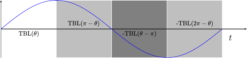 |
We’ll leave the first section alone. This will become our quarter-wave sinewave table. The second section is identical to the first, only in a backwards order. Hence, if we reverse our index, we should be able to recover anything from this quarter wave of the table. The third and fourth sections are identical to the first two, only their results will need to be negated afterwards.
Since we are splitting the full wavelength into four sections, the top two phase bits can be used to determine which of the four sections we are in. If the most significant bit is set, then we’ll want to negate the result. If the next significant bit is set, we’ll want to read backwards out of the table.
This quarter wave table runs into a bit of a problem with phase quantization, though. Consider a phase quantized table with only 16 entries, such as shown in Fig 2.
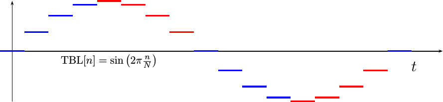 |
This table has lost the symmetry that was originally present in the sinewave. In particular, table[4]’s value is not present in table[0:3]. If we were to use table[3] to represent the missing table[4] value, we might get a sinewave looking like Fig 3. below.
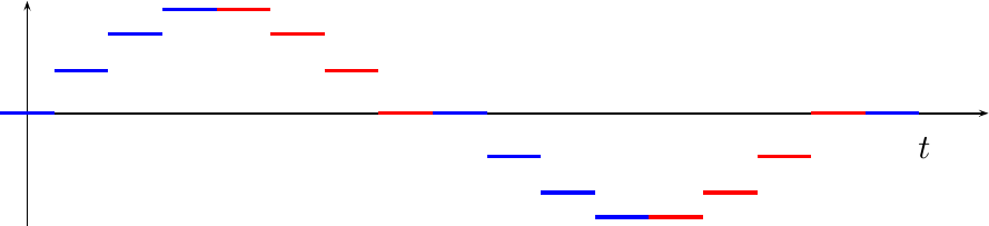 |
Notice how flat the sinewave is every time it crosses zero. It’s not supposed to be this flat. The slope of a sinewave is supposed to be at a maximum when it crosses zero–not flat. This shape distortion will create harmonics that we are not expecting if we don’t fix it.
If we instead advance the sinewave table entries by a half of a sample of phase each, the result will have less harmonic distortion. (i.e., it’ll be closer to the right shape, even if shifted left a touch). The result would then look like Fig 4.
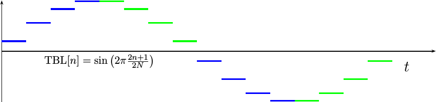 |
The resulting equation for this table is also shown in Fig 4.
The algorithm we want to build will take the first quarter of this sinewave, place it into a table, and then use that same table to generate the other four quarters of the wavelength.
Building the Algorithm
It’s now time to build this algorithm. Although the algorithm itself is quite simple, I’m going to build it in stages and use this as an opportunity to discuss how to build a pipelined algorithm in general. This will allow us to compare several different implementations, and judge between good an bad approaches.
Our first draft for this algorithm uses a giant case statement:
always @(posedge i_clk)
begin
	case({ i_phase[(PW-1):PW-2] })
	2'b00:	o_val <=  tbl[ i_phase[(PW-3):0]];
	2'b01:	o_val <=  tbl[~i_phase[(PW-3):0]];
	2'b10:	o_val <= -tbl[ i_phase[(PW-3):0]];
	2'b11:	o_val <= -tbl[~i_phase[(PW-3):0]];
	endcase
end
In this piece of code, i_phase is the input
phase
request, tbl is the quarter wave
sinewave
table, and o_val is the output
sinewave.
PW is the
phase
width, or equivalently the number of bits in i_phase.
You may notice that I haven’t used TBLLEN/4-1-i_phase at all when reversing
the table entries. Instead, ~i_phase accomplishes the same effect. To know
why this is relevant, remember the two steps to negating a two’s complement
number: invert all the bits and add one. In this case, we’d subtract one
after adding one, so we can just invert the bits. As an example, then, if
i_phase counts from 0 to 15, ~i_phase would count from 15 back down to 0.
The problem with this big case statement approach is that most block RAMs are very particular about how they are accessed. Extra logic on the index is not allowed, neither is extra logic on the output. Adding logic in either place can interfere with the synthesis tool and keep it from recognizing your table as a block RAM (or ROM in this case). When dealing with this, I have found the following form to be reliable among the various hardware’s I have worked with.
always @(posedge i_clk)
	if (i_ce)
		tblvalue <= tbl[index];
Perhaps this is simpler than it needs to be, but it does work across vendors’ tool-suites.
This may also be the time to discuss our pipeline strategy. Looking over the
various pipeline
strategies
we posted about earlier, this already looks like the beginning of the
“global CE” approach. If we look up the examples of where the “global CE”
pipeline strategy makes the most sense, you may recall that
DSP
logic was one of the common applications of this approach. Since that’s what
we are building today, we’ll keep the i_ce
line, and add it into the rest of our logic.
Working the simplicity of this block RAM access into our logic, though, will take some work. We’ll need to spend a clock to calculate the index, and another clock after that to deal with the negation.
This brings us to our second approach to our logic.
always @(posedge i_clk)
if (i_ce)
begin
	// First, calculate the table index
	if (i_phase[(PW-2)])
		index <= ~i_phase[(PW-3):0];
	else
		index <=  i_phase[(PW-3):0];

	// Use the index to access Block RAM
	tblvalue <= table[index];

	// Handle the negation afterwards
	if (i_phase[(PW-1)])
		o_val <= -tblvalue;
	else
		o_val <=  tblvalue;
end
This approach still has some hazards to it. Perhaps if we drew a data flow diagram, such as Fig 5 below, these hazards will become be more apparent.
 |
Let’s work with this flow diagram for a moment. First, it helps to
separate the data flow variables into clock transitions regions. (We’ll
show this in Fig 6 below in a moment.)
i_phase would be in the first clock. We’ll call this the input clock.
index is in the next clock, etc. Once you separate these variables, then
you can see the problem with the negation logic. This negation flag
needs to come from the
high bit of i_phase[(PW-1)], but it has to be available after the table
look up. To make this problem more apparent, draw vertical lines through
the diagram, dilineating the processing clocks. Data flows should not cross
through such lines, without being clocked into a new register–else you’ll
have a pipeline bug.
The solution to this problem is to schedule the pipeline logic.
Specifically, we’ll create a register to hold i_phase[(PW-1)] while
the table index is calculated and the table value is looked up. We can
implement this with a two stage shift register, captured by negate[0] and
negate[1]:
always @(posedge i_clk)
if (i_ce)
begin
	negate[0] <= i_phase[(PW-1)];
	// ...
	negate[1] <= negate[0];
	if (negate[1])
		// ...
end
A new data flow diagram for this modified algorithm might look like Fig 6.
 |
Notice how each variable is now associated with a clock period in the pipeline.
Written out, our logic now looks like:
// Initialize the quarter-wave table
initial	$readmemh("quarterwav.hex", quartertable);

always @(posedge i_clk)
	if (i_ce)
	begin
		// Clock one
		negate[0] <= i_phase[(PW-1)];
		index  <= i_phase[(PW-2)]
				? ~i_phase[(PW-3):0]
				:  i_phase[(PW-3):0];

		// Clock two
		negate[1] <= negate[0];
		tblvalue <= table[index];

		// Output clock
		if (negate[1])
			o_val <= -tblvalue;
		else
			o_val <=  tblvalue;
	end
You can also find a full example of this logic here.
At this point, we are almost done. All that’s left is to create a hex file to be used to crate this table. This can be done from a simple C++ program, where the relevant portion is shown below:
int	tbl_entries = (1 << lgtable),
	maxv = (1 << (ow-1))-1;

for(int k=0; k < tbl_entries/4; k++) {
	double	dv, ph;
	ph = 2.0 * M_PI * (double)k / (double)tbl_entries;
	ph+=       M_PI             / (double)tbl_entries;
	dv = maxv * sin(ph);

	if (0 == (k%8))
		fprintf(hexfp, "%s@%08x ", (k!=0)?"\n":"", k);
	fprintf(hexfp, "%0*x ", (ow+3)/4, (int)(dv) & ((1<<ow)-1));
} fprintf(hexfp, "\n");
Well, not quite. The problem with this approach is that the table generator is closely associtated with the Verilog code itself. In particular, you can’t change the number of table entries, or for that matter the width of the table entries, without also adjusting the Verilog code. For this reason, the C++ generator program creates both the Verilog code and the hex table at the same time.
That’s it! We’ve now made a sinewave generator from just a quarter wave table. We’re still going to need to come back to test this table, to build a test bench and prove that it works, but that’s the basics of the algorithm.
Conclusion
This post is one in a small series of posts discussing how to generate a sinewave. We’ve already discussed a very simple sinewave generator, and we are well on our way to creating and explaining a full blown CORDIC sinewave implementation.
These sinewave generators will then form the basis for testing the digital filters that I intend to discuss and demonstrate as well.
So, while this is the end of this post, in many ways it is only one step forward in building Digital Signal Proccessing algorithms within an FPGA. Stick around, there’s a lot you can do with a sinewave.
But he went out, and began to publish it much, and to blaze abroad the matter, insomuch that Jesus could no more openly enter into the city, but was without in desert places: and they came to him from every quarter. (Mark 1:45)