
Building a Downsampling Filter
Some time back, I asked my Patreon sponsors for topics they’d be interested in reading about. One particular request was to discuss how to put all the pieces together into a DSP design. Since I had a nice open-source FFT demonstrator–a basic spectrogram display–I thought that might make a nice example to work with.
If you look at that project, you might be surprised at how easy it is to read the data flow through the main verilog file. As shown in Fig. 1 below, the data flow follows a very linear series of steps.
 |
It starts with a analog to digital converter, in this case from a Digilent PMod that produces data at 1Msps. Since this is still way too fast for a spectrogram operation, the data is sent into a downsampler–the topic of today’s discussion. Coming out of the downsampler, the data goes either into a traditional FFT window function or a fancier window with (almost) no spectral leakage. From there, the data passes through an FFT, the logarithm of the complex output magnitude squared is calculated, and then everything gets written to memory. The final step, drawing the results to the screen, is somewhat of an icing on the cake.
Let’s set ourselves as a goal understanding how this design works. We’ve already discussed how to build a VGA display controller, although we may also choose to come back in order to discuss it’s HDMI cousin along the way. We’ve also discussed the asynchronous FIFO that’s used to feed this VGA controller, and the FFT that forms the center of the operation. We’ve also discussed the Wishbone to AXI bridge that I use to make DDR3 SDRAM access easy to work with.
Other fun topics we might discuss include the FFT window function, or how the display was put together so as to give the appearance of a horizontally scrolling raster. (Vertical scrolling would’ve been easier.) Perhaps the more important components are the A/D controller, and the framebuffer “memory to pixel” controller.
Today, though, I’d like to discuss the downsampler.
Yes, we’ve discussed filtering before. We’ve even gone over several filtering implementations. [1] [2] [3] [4] [5] [6] [7] [8] That said, we haven’t really discussed how to integrate formal verification in DSP designs. Nor have we discussed how to handle multiple signaling rates. I’d also like to discuss the ever present scaling problem, but at this point I’m not sure I have a good solution to offer for it.
But we’ll get to all that.
For now, let’s start with the downsampler.
Downsampling
At it’s most basic, a
downsampler
is a logic block that takes a signal sampled at one rate and
resamples it at a
lower rate. This can be as simple as just
picking every Nth sample. You can also get fancy and interpolate between
sample points, and
downsample
by some rational amount such as 16368/2048 (a common
GPS
problem). Since this is really my first post on the topic of
downsampling,
we’ll stick to the every Nth sample variety.
 |
For such a simple
downsampler,
we might initially describe the operation as simply taking one point out of
every D points,
 |
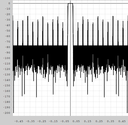
Of course, there are problems with this easy solution in practice. The biggest of these problems is “aliasing”. Perhaps you may remember the problem with aliasing from the demonstration of the “improved” PWM implementation. In that implementation, a single up-swept tone input also produced a tone sweeping in the other direction.
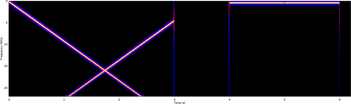 |
Note that the zero frequency is (unconventionally) at the top of Fig. 3, so an upswept tone appears as a diagonal line from the top (zero frequency) left (zero time) corner.
The aliasing problem was worse when we didn’t use a resampling filter. In this case, the single swept tone input appeared to produce multiple swept tones in what appeared to be a crosshatch pattern on the spectrogram.
 |
In that application, we were upsampling and not downsampling, but the principle is still the same: out of band signals might alias in-band if we aren’t careful.
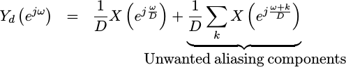
To see this mathematically, imagine we have an incoming signal which consists of a complex exponential.
 |
If you just
downsample,
this signal, picking every D‘th sample, then
this exponential
will now exist in many places of the resulting spectrum.
 |
If on the other hand we first convolve our signal with some kind of “filter”,
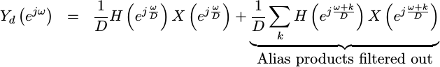 |
we can now use the filter to control how much of this exponential ends up in our result.
 |
Indeed, the only way to make certain that the
downsampled
signal,  ,
contains only the spectral content from the band of interest is to
filter out all of the other
,
contains only the spectral content from the band of interest is to
filter out all of the other
 bands. For this
reason, the downsampling
operation
needs to be coupled with a
filter
operation as well, as shown in Fig. 5.
bands. For this
reason, the downsampling
operation
needs to be coupled with a
filter
operation as well, as shown in Fig. 5.
With a proper filter before our downsampler, we can mitigate the problems associated with aliasing.
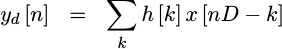
Operationally, this would look like Fig. 5 above. We might write the two steps as,
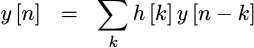 |
- Select every
D'th output sample
 |
Sadly, filters
can be expensive to
implement, and good
filters
all the more so. The filtering
operation associated with a
downsampler,
however, is a special case since we don’t really care about every outgoing
sample. We only care about every Dth sample. A smarter
implementation
might calculate just these outputs, and spare us from the heavy computational
burden of calculating results we aren’t going to use.
Here’s the problem: my cheapest filter so
far can only accomplish a
 tap filter if the data rate is
 to begin with. In
the case of the above FFT demonstration
design,
the system clock is 100Mhz, and the incoming sample rate is 1MHz. If I used
this cheap filter,
I would only ever be able to implement a 200 tap filter.
to begin with. In
the case of the above FFT demonstration
design,
the system clock is 100Mhz, and the incoming sample rate is 1MHz. If I used
this cheap filter,
I would only ever be able to implement a 200 tap filter.
 |
My spectrogram design, required a 1023 tap filter followed by a 23:1 downsampler in order to get the -80 dB out-of-band rejection I wanted. A 200 tap filter would never cut it.
On the other hand, what if we built something like the cheap filter we built
before, but this time
engineered it so that it only produced those values that we were going to keep?
Hence, we we’d only calculate values
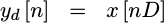
![y[nD]](/img/fftdemo/eqn-ynd.png) (for all values of
(for all values of n), rather
than the unused values such as
![y[nD+1], y[nD+2]](/img/fftdemo/eqn-unused-series.png) , etc.
We could do this if
we merged the downsampler and the filter
together,
as in:
, etc.
We could do this if
we merged the downsampler and the filter
together,
as in:
 |
Using this method, I could then implement a 2300 tap filter as we’ll discuss below–even though my design only required a 1023 tap filter.
Slow Filters (Implementation Overview)
This downsampler follows a particular class of filters I call “slow filters”. What makes them slow is that they are area optimized, rather than throughput optimized. The goal of these “slow” filters is to do the entire operation using a single, multiplexed, hard multiplication element. This will also restrict how fast data can be given to the filter. By contrast, I’ve used the term “fast” filter to describe a filter that can handle a new data value every sample. Such “fast filters” often require as many hard multiplication elements as they have coefficients. Of course, compromises exist between these two extremes–but that’s another topic for another day.
Indeed, my initial filter designs were all focused around “fast filters”. [1] [2] [3] That was before I tried working with audio on Lattice’s iCE40 chips. Suddenly my entire “fast filter” library was too expensive for the applications I needed, and I needed to spend some time building filters that didn’t use as many hard multiplies.
The fascinating part about slow filters is that they all have almost exactly the same structure–although with subtle variations from application to application. Data comes in, gets written to memory, memory and coefficient indexes are calculated, data and coefficient values are read from memory, products get calculated and then accumulated into a result. On a clock by clock basis, this looks like:
- Wait for and then accept a new data value when it becomes available, write it to memory, and adjust the memory write index
- Read one value from data memory and one value from coefficient memory. Adjust the read-memory indexes.
- Multiply these two values together
- Accumulate the results together
- Round the accumulated value into a result, and set a flag when it’s ready.
For reference, Fig. 7 below was the figure we used when explaining this operation before.
 |
Coefficient Updates
If your goal is to build the
fastest and cheapest
digital filter out
there, then updating the coefficients post-implementation is a bad thing: it
prevents a lot of synthesis optimizations that might otherwise take place. For
example, multiplies by constant zeros could be removed, by constant 2^n
values can be replaced with shifts, and 2^n+2^k values can be replaced
with shift and adds.
The problem with doing this is that if you want to build a generic filter, and then to discuss how much area a generic filter would use, or even to test a generic filter on a test bench with multiple coefficient sets, then you need an interface that will allow you to update the coefficients within your filter.
 |
Years ago, when I built my first FPGA filter, I created a filter with over a thousand elements for which the coefficients could be accessed and read or written using a Wishbone bus interface. At the time, I thought this would be the ideal interface for adjusting filter coefficients. I was then rudely awakened when I tried to implement this design on an FPGA.
The problem I had was specifically that in order to implement each of the multiplies in hardware in parallel at the same time, all operating on the same clock cycle, all of the filter coefficients have to be present in FFs at the same time. The memory interface then created a series of 1024 10-bit decoders and a 1:1024 demultiplexer–one for each bit of the coefficients–and that was just the write half. Sorry, but such a “beautiful” interface isn’t worth the logic cost. (I’m not sure I could’ve afforded the board it would’ve taken to make this work at the time.)
 |
A simpler interface is to use a series of shift registers, together with a flag indicating when to update the FPGA with a new coefficient. If done properly, this won’t cost anything more than the number of FFs you already need to hold the coefficients in the first place.
While we don’t need to use this shift register implementation with a typical “slow filter”, it still forms the motivation the interface we’ll use today. Writes to the coefficient “port”, a memory port occupying only a single address on the bus, will write new values to the coefficient memory. Resetting the core will reset the write pointer to the beginning of coefficient memory. That way we can reset the core and then write the coefficients to it one at a time. Even better, any bus interface wrapper that works for “fast” filters will also work for our “slow” filters.
Implementation in Detail
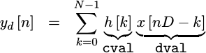
At this point, implementing a downsampling filter should be fairly straightforward. We’re just implementing a straightforward equation.
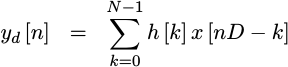 |
We’ve gone over the basic sections of such a filter, and we’ve outlined roughly how the algorithm works. All that remains is to walk through the actual logic, and see how it gets accomplished in detail below. Then, in the next section, we’ll discuss how formal methods might help verifying a structure like this one. For those interested in following along within the design itself, I’ll be working through this version of the downsampling filter implementation below.
The filter itself starts out with a declaration of the parameters that can be used to control the implementation of the core.
This includes specifying the widths of the input, the output, and the
coefficients, as well as what our downsample rate is–what we called D
above.
module	subfildown #(
		//
		// Bit widths: input width (IW),
		parameter	IW = 16,
		// output bit-width (OW),
				OW = 24,
		// and coefficient bit-width (CW)
				CW = 12,
		//
		// Downsample rate, NDOWN.  For every NDOWN incoming samples,
		// this core will produce one outgoing sample.
		parameter	NDOWN=5,
		// LGNDOWN is the number of bits necessary to represent a
		// counter holding values between 0 and NDOWN-1
		localparam	LGNDOWN=$clog2(NDOWN),
The next section controls our initial coefficient loading, ultimately ending
with the INITIAL_COEFFS parameter that names a file containing the
coefficients to be used in the filters implementation.
		//
		// If "FIXED_COEFFS" is set to one, the logic necessary to
		// update coefficients will be removed to save space.  If you
		// know the coefficients you need, you can set this for that
		// purpose.
		parameter [0:0]	FIXED_COEFFS = 1'b0,
		//
		// LGNCOEFFS is the log (based two) of the number of
		// coefficients.  So, for LGNCOEFFS=10, a 2^10 = 1024 tap
		// filter will be implemented.
		parameter	NCOEFFS=103,
		localparam	LGNCOEFFS=$clog2(NCOEFFS),
		//
		// For fixed coefficients, if INITIAL_COEFFS != 0 (i.e. ""),
		// then the filter's coefficients will be initialized from the
		// filename given.
		parameter	INITIAL_COEFFS = "",
You’ll notice that I tend to make a liberal use of localparams above. They
are very useful for creating parameter-like structures of derived values that
cannot be overridden from the parent context. My only problem with using
localparams has been that Icarus Verilog’s
support is more recent than the version provided for my current flavor of
Ubuntu. You might find, therefore, that you need to upgrade Icarus
Verilog to the latest
version from source and use the -g2012 option to get access to this feature.
Let me also caution you when using $clog2() to calculate the bit-width
required of a given value: the $clog2() result will produce the bitwidth
necessary to contain a value between zero and the value minus one–not the
bit-width necessary to maintain the value itself. If this is a problem, you
can add one to the argument of the $clog2 value, as in $clog2(A+1). I’ve
had no end of this problem when working with
AutoFPGA, however in today’s
example
$clog2 will work nicely as is.
There is, however, one parameter in today’s
example
that I’ve been burned by, and worse I’m not quite sure the right answer at this
point, and that is the SHIFT parameter. At issue is, how shall the design
go from the bit width of the accumulator to the outgoing bitwidth? The easy
answer is to drop any bits below the desired amount, or perhaps to round to
a nearby
value. (Beware of overflow!)
The problem with this answer is that your filter
coefficients might be such
that the maximum value will never be reached. In that case, you’ll want to
multiply the accumulator’s result by a power of two in order to
recapture some dynamic range
and get it into the range that you want. This is the purpose of the SHIFT
parameter below.
parameter SHIFT=2,A SHIFT of two specifies that we’ll multiply the result by 2^SHIFT = 4
before returning the output.
The problem with this parameter, and the problem I’m still mulling over, is
that this definition doesn’t relate very well to the problem definition. If
you run your favorite analysis tools on the coefficients, you can easily
calculate the gain of the
filter
and then a shift to place the results of the
filter
into range. This SHIFT value isn’t that. It’s more like the opposite of
that, and so I’ve been confused more than once at how to set it.
In other words, this portion of the filter is likely to be changed in the future once I figure out a better answer to this problem–something that makes adjusting the scale at the end more intuitive.
The last local parameter is the bit width of our accumulator. This
follows from the bit width of multiplying two values together, one with IW
bits and another with CW bits, and then adding NCOEFFS of these values
together.
localparam AW = IW+CW+LGNCOEFFS |
The next step is to define a set of ports appropriate for this design.
When we last discussed how to go about testing a filter, we came up with a
“universal” filter port set.
This port set included the more obvious clock and reset, as well as a incoming
data port. When the incoming i_ce signal was true, new data was available
on that port. There was similarly an i_tap_wr signal to indicate that we
wanted to write a new coefficient value (tap) into the coefficient shift
register. Using this approach, we could apply a new value on every clock
cycle to this filter.
 |
This downsampling
filter has
to be different, specifically because the i_ce
signal
would be inappropriate for driving a sample stream at one Dth the incoming
rate. Instead, this
filter
has an outgoing sample valid signal,
o_ce,
as shown in Fig. 11. Indeed, that’s probably the biggest difference in ports
between this downsampling
filter
and the filters we’ve built
before.
Enough of the preliminaries, let’s look into how this filter is implemented.
The first step is to initialize our coefficients.
	generate if (FIXED_COEFFS || INITIAL_COEFFS != 0)
	begin : LOAD_INITIAL_COEFFS

		initial $readmemh(INITIAL_COEFFS, cmem);

	end endgenerate
Note that the generate will always load a filter any time FIXED_COEFFS is
set. This should force an error if the file isn’t defined. Of course, if the
file INITIAL_COEFFS is defined, we’ll always load the coefficients from that
file. Otherwise, they’ll be need to be loaded across the bus since their
initial values would be implementation dependent upon startup.
Above I said that the ideal method for adjusting filter coefficients was
a shift register implementation. Such an implementation would require an
update flag, herein called i_tap_wr, together with the new value, i_tap.
That interface works great for a shift register implementation, but the optimizations used by this filter require that the coefficients be kept in a block RAM, rather than in registers. So, instead, we’ll keep track of an index register. We’ll set the index register to zero on any reset, but otherwise increment it with every write. Likewise, on every write we’ll write our value to memory at the index given by the index register.
	generate if (FIXED_COEFFS)
	begin : UNUSED_LOADING_PORTS
		// ...
	end else begin : LOAD_COEFFICIENTS
		// Coeff memory write index
		reg	[LGNCOEFFS-1:0]	wr_coeff_index;

		initial	wr_coeff_index = 0;
		always @(posedge i_clk)
		if (i_reset)
			wr_coeff_index <= 0;
		else if (i_tap_wr)
			wr_coeff_index <= wr_coeff_index+1'b1;

		always @(posedge i_clk)
		if (i_tap_wr)
			cmem[wr_coeff_index] <= i_tap;

	end endgenerate
The second major block of this
filter is
where we write the data samples into memory. On every new sample, marked by
the incoming clock enable
line
i_ce we adjust our write address and write one sample to memory.
	initial	wraddr    = 0;
	always @(posedge i_clk)
	if (i_ce)
		wraddr <= wraddr + 1'b1;

	always @(posedge i_clk)
	if (i_ce)
		dmem[wraddr] <= i_sample;
One of the implementation keys that often surprise individuals is that block RAM cannot be reset. If you make the mistake at this point, therefore, and try to re-initialize the block RAM on any reset, you’ll be disappointed to find that the data memory will no longer be implemented in block RAM. Indeed, it might no longer fit on your chip. For more information on what assumptions may be assumed of block RAM, feel free to check out the block RAM lesson from my beginner’s tutorial.
In most cases, this isn’t usually a problem–the filter will glitch following
any reset, but then it will settle out. If it becomes a problem, you can
add some circuitry to the outgoing CE signal to prevent CE generation until
enough data values have been set–effectively skipping the filter’s runup.
This did became a problem for me at one time when trying to figure out how to
properly reset a filter of this type to a known configuration for
simulation
testing. The solution I picked for my test bench was to just hold
i_reset and i_ce high while holding i_sample at zero for
(1<<LGNCOEFFS) cycles. As you’ll see later, holding i_reset high prevents
any outputs from being generated. This approach allowed me to reset the data
memory–even if it requires some external work to get there.
Since we’re implementing a
downsampling
filter, we will be accepting D
(NDOWN) samples into our filter for every sample out we produce. That means
one of every D samples entering our
design
will trigger the processing necessary to create a new output sample. To know
when a given incoming sample is the one that will trigger the processing for
new output, we’ll need to implement a counter. This particular counter
implementation is a count down counter, counting down from NDOWN-1 to zero,
and at zero we set the first_sample flag to indicate that the next incoming
sample will start our processing run.
	initial	countdown = NDOWN[LGNDOWN-1:0]-1;
	initial	first_sample = 1;
	always @(posedge i_clk)
	if (i_ce)
	begin
		countdown <= countdown - 1;
		first_sample <= (countdown == 0);
		if (countdown == 0)
			countdown <= NDOWN[LGNDOWN-1:0]-1;
	end
The next step is to read from our memories–the data memory and the coefficient memory. Getting there, however, requires that we know the memory indexes we need to read from.
Our first step towards calculating the two indexes we need is to calculate
when we are on the last coefficient of our filter and so need to stop our
operation. The last coefficient will be marked as NCOEFFS-1, but we’d like
to set this flag one clock earlier–leading to the logic below.
	initial	last_coeff = 0;
	always @(posedge i_clk)
		last_coeff <= (!last_coeff && running && tidx >= NCOEFFS-2);
So, here’s how it works: when the first sample of a set comes in, our
coefficient index will be 0. We’ll then increment that coefficient index,
tidx (read tap index) on every clock cycle until it gets to NCOEFFS-1.
Along the way, we’ll use a flag, running, to indicate that we are running
through that coefficient list. Then, on that cycle, last_coeff will be
true and we can stop running.
When we’re not running, we’ll hold running at zero–up until the first
incoming sample (i_ce).
	initial	tidx = 0;
	initial running = 0;
	always @(posedge i_clk)
	if ((!running)&&(!i_ce))
	begin
		tidx <= 0;
		running <= 1'b0;
	end else if ((running)||((first_sample)&&(i_ce)))
	begin
		if (last_coeff)
		begin
			running <= 1'b0;
			tidx <= 0;
		end else begin
			tidx <= tidx + 1'b1;
			if ((first_sample)&&(i_ce))
				running <= 1'b1;
		end
	end
You’ll note that I haven’t used a reset here. I’m going to contend that it’s
not necessary. Even in a design requiring a reset, where the initial values
are ignored, the running and tidx (coefficient index) flags will settle
into their appropriate values within 2*NCOEFFS clocks. If you really want
a reset, you could add it to the first if statement above.
What happens if the first sample comes in and the design was already running
with the last set of NDOWN incoming samples? Simply, the design would no
longer function as designed. Sure, it would still produce outputs, but they
would be based upon the wrong coefficient indices. It is the responsibility
of the surrounding environment to make certain this assumption isn’t broken.
We must issue the last coefficient index before the first sample of the
next set. Once the design stops running, it will then wait for an incoming
sample where first_sample is also set before starting its next
run–guaranteeing that we’ll end up synchronized even without a reset.
The data memory index, didx, is very similar to the coefficient index above.
The difference is that the data memory index doesn’t get reset at the beginning
of every run. Instead, when we aren’t running, the data index gets set
to the index of the next data to be accepted into the core. On the clock
cycle that data is accepted, we’ll read from what used to be there. That
will then be the oldest data.
initial didx = 0;
always @(posedge i_clk)
if (!running || last_coeff)
// Waiting here for the first sample to come through
didx <= wraddr + (i_ce ? 1:0);
else
// Always read from oldest first, that way we can rewrite
// the data as new data comes in--since we've already used it.
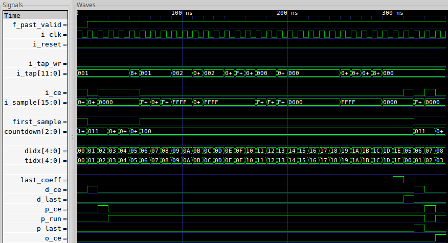
didx <= didx + 1'b1;In case you are starting to get lost in the words here, it might help to have a trace to see what’s going on. Therefore, here’s a possible trace showing what might be expected at this point in our implementation.
 |
This trace has been built for a subsample size of D=5 and a filter length of
NCOEFFS = N = 31. As you can see, the run is triggered by the first sample of
D arriving. From that point on, the core runs through its coefficient set
and past data. Once complete, last_coeff is set and the design sets up for
the next run. As part of a separate pipeline, D values are accepted and then
first_sample is set high. These can arrive at any speed, subject to the
requirement that no more than D samples can be accepted mid run. Then, once
first_sample is set, the next data sample coming in starts a new run. It’s
important that this next sample not arrive until the run has complete.
Perhaps this core should also have a ready
output, perhaps even !running || !first_sample, but I haven’t needed to
attach such a ready input (yet).
Now that we have indices for both data and coefficient memories, we can now read their values from their respective block RAM’s.
	always @(posedge i_clk)
	begin
		dval <= dmem[didx];
		cval <= cmem[tidx];
	end
If you look back at the formula we are implementing, we now know what
h[k] and x[nD-k] portions of our convolution product are.
 |
The next big steps will be to multiply these two values together, and then to accumulate their result into a sum to create our output.
Before leaving this initial clock cycle and launching into our pipeline, there’s two other required steps. First, we’ll need to track the initial sample through our pipeline to know when to generate an outgoing sample. Second, we’ll need to generate a flag to tell us when to accumulate a new value, versus when to clear our accumulator.
By way of introducing the values we need for keeping track of this pipeline, let me diagram out the pipeline itself in Fig. 13.
 |
This pipeline is really driven by the time it takes to read from block RAM, the time it takes to form a product, and the time it takes to sum the results. Each of these tasks takes one clock, and there’s no real easy way to speed this up other than pipelining the processing as shown in Fig. 13 above. The figure shows a first stage where the indexes are calculated. At the same clock cycle indexes are valid, the new sample may arrive. One clock later, the data are available from the block RAM memory reads above. One clock later, the product is complete. That will be our next step, once we finish up with the signaling here. Once the product is available, we’ll enter into first an accumulator stage and then the output stage.
As the first stage has an i_ce value to kick it off, I also use a d_ce
value to capture that cycle of the first sample as it exists after the
data are read and d_last to capture the last valid data cycle. In a similar
vein, only one clock later, p_ce will capture the first cycle where the
product is valid and p_last will capture the last one. There’s also the
p_run signal, used to tell the accumulator when to accumulate versus
reloading from the product result. This p_run signal will get set by
p_ce, and then again cleared by p_last. So let’s
quickly discuss these five registers, d_ce, d_last, p_ce, p_last,
and p_run.
We’ll skip the reset preliminaries for these registers. Basically, all of these five flags get cleared on any reset.
	initial	d_ce  = 0;
	initial	p_run = 0;
	initial	p_ce  = 0;
	initial	d_last= 0;
	initial	p_last= 0;
	always @(posedge i_clk)
	if (i_reset)
	begin
		d_ce  <= 0;
		p_ce  <= 0;
		p_run <= 0;
		d_last  <= 0;
		p_last  <= 0;
	end else begin
As mentioned above, d_ce describes when the data stage has the first valid
value within it.
d_ce <= (first_sample)&&(i_ce);d_last describes the last clock cycle with valid data within it. This is
easily set based upon the last_coeff register we set earlier.
d_last<= last_coeff && p_run;p_ce follows after d_ce one cycle later, to indicate when the
multiplication product has its first valid output.
p_ce <= d_ce;p_run is just a little
different. Instead of referencing the first item in the run, p_run will
be true for all subsequent valid products. It gets set on the cycle after
p_ce, and gets cleared by the last product. The result is that p_run can
be used later to indicate when it’s time to accumulate into our accumulator.
p_run <= !p_last && (p_run || p_ce);The last product itself, noted by p_last, is valid one clock cycle after the
last data value. This value needs to be gated by p_run, however, or a
reset mid-run might throw the whole cycle off.
		p_last<= p_run && d_last;
	end
If this seems confusing, then perhaps Fig. 14 below will help clear things up.
 |
Here you can see that p_ce is true on the first clock cycle where the product
is valid. That will be our signal to reload the accumulator with an initial
value. After that clock cycle, we’ll hold p_run high for another N-1
cycles, before resetting as part of the next cycle. Here you can see how
p_last is our signal to reset p_run. Further, you can compare the running
signal to p_run. The two signals are identical, save for a
two cycle delay–caused by propagating the signal through the pipeline. The
other check, to make sure we’ve done this right, is to make certain that
the number of cycles where p_ce || p_run are true are equal to the number
of coefficients in our filter.
We can now calculate the product of data sample with our coefficient.
	(* mul2dsp *)
	always @(posedge i_clk)
		product <= dval * cval;
This forms the product portion of the formula we are trying to implement.
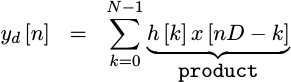 |
At this point I need to introduce one more signal, acc_valid. The problem
with our current setup is that the signal for o_ce to become valid is when
the first product is true. That will be the same cycle the accumulator is
cleared, so it’s a perfect time to copy the value to the output. What happens,
though, if we haven’t run through our summation at that time? For this reason,
I use a quick and simple flag I call acc_valid. If acc_valid is true,
then on the first product when I would clear the accumulator, I can also
generate an output sample from the accumulator.
To make this work, I’ll reset acc_valid on any reset. If we ever add
anything to our accumulator, then there will be a valid amount in the
accumulator and so I can then set acc_valid. I can now use
this to gate when o_ce should be set or not in another step or two.
	initial	acc_valid = 0;
	always @(posedge i_clk)
	if (i_reset)
		acc_valid <= 0;
	else if (p_run)
		acc_valid <= 1;
If I later decide that it’s important to keep the
filter
from glitching following a reset, I could come back and add a counter to this
acc_valid register–forcing NCOEFFS inputs before setting the first
acc_valid.
The next task is to form our sum. Using the p_ce flag, to indicate the
first product in the run, and the p_run flag, indicating that more
accumulation is necessary, this gets really easy. On a p_ce cycle, we
set the accumulator to the result of the product, and on any p_run cycle
we add the new product to the prior accumulator value.
	initial	accumulator = 0;
	always @(posedge i_clk)
	if (i_reset)
		accumulator <= 0;
	else if (p_ce)
		// If p_ce is true, this is the first valid product of the set
		accumulator <= { {(LGNCOEFFS){product[IW+CW-1]}}, product };
	else if (p_run)
		accumulator <= accumulator
			+ { {(LGNCOEFFS){product[IW+CW-1]}}, product };
Now that we have our result, let’s adjust the number of bits in it.
So far, our product has AW bits in it. That’s the IW+CW bits
required to hold a product of values having IW and then CW bits,
together with an additional LGNCOEFFS bits to account for adding NCOEFFS
of these products together.
The good news of this AW=IW+CW+LGNCOEFFS number is that it is guaranteed
never to overflow. If
we just grab the top OW bits, our output bit-width,
we are guaranteed not to have overflowed. That’s the good news. The bad news
is that it is a very conservative width, and may well be many more bits than are
truly necessary to hold the result. The result of just grabbing the top
OW bits may then reduce our precious
dynamic range.
For this reason, I’ve introduced the SHIFT parameter above. We’ll now
shift our signal left by SHIFT bits before rounding and grabbing the result.
	generate if (OW == AW-SHIFT)
	begin : NO_SHIFT
		assign	rounded_result = accumulator[AW-SHIFT-1:AW-SHIFT-OW];
	end else if (AW-SHIFT > OW)
	begin : SHIFT_OUTPUT
		wire	[AW-1:0]	prerounded;

		assign	prerounded = {accumulator[AW-SHIFT-1:0],
						{(SHIFT){1'b0}} };
		assign	rounded_result = prerounded
				+ { {(OW){1'b0}}, prerounded[AW-OW-1],
					{(AW-OW-1){!prerounded[AW-OW-1]}} };
	end else begin : UNIMPLEMENTED_SHIFT
	end endgenerate
Sadly, after using the logic above many times, I kept running into overflow problems. My answer to “overflow” when designing this core was that it was the responsibility of the designer to keep overflow from happening. Unfortunately, as the designer using the core, it became difficult to just look at a trace and know that a particular problem was the result of overflow. Therefore, I came back to this design to retro-fit it for overflow detection.
The key to overflow detection is to check the sign of the result from before shifting and compare it to the sign bit afterwards. If the two disagree, there’s been an overflow.
	generate if (OW == AW-SHIFT)
	begin : NO_SHIFT
		assign	sgn = accumulator[AW-1];
		assign	rounded_result = accumulator[AW-SHIFT-1:AW-SHIFT-OW];
		assign	overflow  = (sgn != rounded_result[AW-1]);
Sadly, when I tried this same approach on the section where I rounded the data to the nearest value, I was surprised to see the result glitching every now and then.
	end else if (AW-SHIFT > OW)
	begin : SHIFT_OUTPUT
		wire	[AW-1:0]	prerounded;

		assign	prerounded = {accumulator[AW-SHIFT-1:0],
						{(SHIFT){1'b0}} };

		assign	sgn = accumulator[AW-1];
		assign	rounded_result = prerounded
				+ { {(OW){1'b0}}, prerounded[AW-OW-1],
					{(AW-OW-1){!prerounded[AW-OW-1]}} };
		assign	overflow  = (sgn != rounded_result[AW-1]);
The problem is that rounding a value between -1/2 and 0 up to 0 will trigger a sign change. “Correcting” this change under the assumption that the correct result should be a maximum negative value rather than leaving it alone was creating glitches I wasn’t expecting.
My solution is a two-fold check for overflow. If the original value is negative, and it becomes positive as a result of the shift, then there was an overflow. On the other hand, if the sign was positive before the shift but became negative after rounding, then there’s been an overflow.
		assign	overflow = (sgn && !prerounded[AW-1])
				|| (!sgn && rounded_result[AW-1]);
Even this isn’t true overflow protection, since we only checked the sign
bit–not all of the SHIFT bits we shifted away. Still, it does get us
that much closer.
What value should the SHIFT be? That follows from the maximum value one
might expect out of the filter, generated by applying a signal consisting of
all maximum values where every value matches the sign of the coefficient
of the filter within. Something like the following expression, therefore,
can calculate our maximum result.
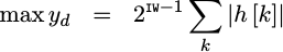 |
Using this result I’d like to be able to specify a shift by,
 |
Unfortunately, my currently chosen SHIFT parameter doesn’t relate to this
ideal formula listed above very well. Indeed, the relationship appears
to be backwards, so I might need to update it in the future.
Let’s continue on anyway. The last and final step of this algorithm is to report the result.
Our result will be valid as soon as the accumulator starts a new sum. At this
point, the accumulator may have been idle for some time. It doesn’t matter.
The accumulator will have the prior sum within it. There’s one exception,
however, and that is if the design was reset mid-run. In that case, the
acc_valid flag will be false telling us not to produce an output this run.
	initial	o_ce = 1'b0;
	always @(posedge i_clk)
		o_ce <= !i_reset && p_ce && (acc_valid);
Nominally our output would simply be the result of rounding and shifting the accumulator.
	always @(posedge i_clk)
	if (p_ce)
		o_result <= rounded_result[AW-1:AW-OW];
However, if multiplying by 2^SHIFT or rounding caused an overflow, then
this is the place to correct for it. In the case of overflow, the correct
answer is either the maximum negative value if the sign were negative, or
the maximum positive value if not. This is an easy check and update.
	always @(posedge i_clk)
	if (p_ce)
	begin
		if (overflow)
			o_result <= (sgn) ? { 1'b1, {(OW-1){1'b0}} }
					: { 1'b0, {(OW-1){1'b1}} };
		else
			o_result <= rounded_result[AW-1:AW-OW];
	end
The fascinating part of this design is how similar it is to other filtering designs I’ve built. [1] [2] [3] They all seem to have (roughly) the same structure, and the same basic steps to their implementation.
Before leaving this implementation section, I should point out that I’ve also built a similar implementation for complex signals, that is–those containing both in-phase and quadrature components. That version is nearly identical to this version, save that it handles two data paths. While I suppose I might have technically just used two versions of this same filter, by combining both paths into a quadrature version, building a quadrature down converter allows me to ensure that the synthesis tool doesn’t infer more logic than necessary.
Formal Verification
When I teach formal verification, one of my early points is that formal methods can’t handle multiplies. The result is that I don’t use formal methods on DSP algorithms–or so I teach. The reality is that there’s a lot to the algorithm above that can be formally verified–just not the product of the multiplication. Not only that, but I’ve gotten to the point where it’s easier to use SymbiYosys to get something up and running than anything else. The reality, therefore, is that you can use formal methods on DSP algorithms–at least enough to get you most of the way there. You’ll still need to do some simulation to be sure the design truly works, but formal methods will get you to that simulation that much faster.
Step one: Replace the multiply
The first step, however, is to replace the multiply. In our case, we’ll replace it with an abstract result–something that might or might not give us the right answer. Any assertions that pass, therefore, would still pass with the right answer.
The key to doing this is to declare a register with the
SymbiYosys
recognized
(* anyseq *) attribute. This will tell the solver that this register
can contain any sequence of values–potentially changing on every clock tick.
These values act like an input port to our routine, only they act like an input
coming into the routine in the middle rather than at the portlist at the top.
As such, the proper constraints for them are assumptions.
(* anyseq *) reg signed [IW+CW-1:0] f_abstract_product;I’m going to constrain my product with just a couple of assumptions. First, the sign of the result must match. Second, anything multiplied by zero must be zero. Third, anything multiplied by one keeps its value. In all other respects, I’m not going to constrain the result of the product at all.
	always @(*)
	begin
		assume(f_abstract_product[IW+CW-1]== (dval[IW-1] ^ cval[CW-1]));
		if ((dval == 0)||(cval == 0))
			assume(f_abstract_product == 0);
		else if (cval == 1)
			assume(f_abstract_product == dval);
		else if (dval == 1)
			assume(f_abstract_product == cval);
	end
Then, instead of setting product = dval * cval, I’ll set it to this abstract
value.
	always @(posedge i_clk)
		product <= f_abstract_product;
This was the approach I used when formally verifying my FFT. In that case, these assumptions were sufficient to be able to reason about the design using a formal solver. In this case, they are overkill since I’m not asserting any properties of either the product, the accumulator, or the resulting output (yet).
Step two: Constrain the inputs
The next step is to constrain the input. In this case, there’s only one
constraint–there can only be D (NDOWN) inputs per run of the
filter.
Until the
filter is
ready for its next set of D inputs, the surrounding environment must wait.
	always @(*)
	if (running)
		assume(!i_ce || !first_sample);
This will keep us from overrunning the filter when using it.
There is a risk here, however. By using a local value within an assertion,
you run the risk that the assertion might prevent proper operation of the
design. We’ll use cover() statement later to make certain that isn’t the
case here.
That’s our only input constraint. Together with the assumptions associated with the abstract multiply above, those are our only assumptions. Everything else is asserted from here on out.
Step three: Generate a quick trace
The next step in getting a DSP algorithm up and running is to generate a quick cover trace.
 |
Depending on the algorithm, such a trace might simply be generated by running a counter and looking for some number of steps from the beginning of time. In the case of one of my polyphase Fourier transform filterbank implementations, a counter was exactly what I needed to get the trace. I counted the number of Fourier transform blocks generated by the filterbank. After seeing two whole blocks, I could examine the core and start making assertions about it.
This design ended up using a simpler approach. In this case, I chose to cover the first output so that I could see the entire operation of this core.
Well, not quite. That alone wasn’t quite good enough. In order to get a trace generated in a short period of time, and moreover one that would fit on my screen, I had to carefully trim down the downsample ratio and filter length. As mentioned above, this example trace is for a downsample ratio of 5:1 and a 31-coefficient filter even though the default filter length and proof is designed for 103 coefficients.
Still, it only takes about 2 lines of formal to get started with a trace that you can then examine to see how well (or poorly) your algorithm is working.
Step four: Start adding assertions
My next step was to work back through the algorithm, looking at every counter within, in order to capture any obvious logic redundancies across values together. While the process is rather ad-hoc, I caught a lot of bugs out of the gate by doing this–still before simulation.
So, for example, the countdown counter should never be greater than NDOWN-1.
	always @(*)
		assert(countdown <= NDOWN-1);
Similarly, the first_sample flag should be equivalent to the counter being
at NDOWN-1.
	always @(*)
		assert(first_sample == (countdown == NDOWN-1));
Moving to the filter index stage, every time I read over the logic for
last_coeff I got confused. I wanted the last_coeff flag to be true
on the last coefficient, so a quick assertion checked that for me.
	always @(*)
		assert(last_coeff == (tidx >= NCOEFFS-1));
Much of the rest of the algorithm is like clock work. If we just keep track of the right values from the right cycles, we should be able to capture everything together.
For example, the data index used within the algorithm is based upon the write address when the first value of the set is written. Let’s capture this value, then, and make assertions about our other values with respect to this one.
	initial	f_start_index = 0;
	always @(posedge i_clk)
	if (i_ce && first_sample)
		f_start_index <= wraddr;
For example, we can count how many items have been written to our filter by comparing this starting index with the current write index.
	always @(*)
		f_written = wraddr - f_start_index;
For example, we can insist that the countdown be equivalent to it’s maximum
value minus the number of values that have been written in this set.
	always @(*)
	if (!first_sample)
		assert(countdown == (NDOWN-1-f_written));
Don’t let the !first_sample criteria fool you: this is really an assertion
for all time. The !first_sample criteria was required to get past the
initial conditions which weren’t quite consistent–nothing more.
A similar assertion can be used to guarantee that we never write more than
NDOWN values per set.
	always @(*)
		assert(f_written <= NDOWN);
One of my big concerns was that I might overwrite a data value mid run. Was the assumption above sufficient to guarantee that the run would be consistent throughout, and only using the data that was there originally? For this, I added another assertion–only this one based on the coefficient index.
	always @(*)
	if ((tidx < NDOWN)&&(running))
		assert(f_written <= tidx);
On the first sample of any set, we should have written either nothing (i.e.
coming from reset), or a full set of NDOWN samples.
	always @(*)
		assert(first_sample ==((f_written == NDOWN)||(f_written == 0)));
I also wanted to make certain that the data and coefficient indices stayed
aligned. As you may recall, the data index starts with the first value
written of the set of NDOWN values, and continues up by one from there whereas
the filter coefficient index starts from zero.
A quick subtraction, subtracting the starting index from the current data index turns this into a number that should match our filter coefficient index.
	always @(*)
		f_dindex = didx - f_start_index;

 	always @(*)
	if (running)
		assert(tidx == f_dindex);
The two steps in this case are important. The first step, the subtraction, wasn’t rolled up into the assertion. That’s because I wanted to guarantee that it was properly limited to the right number of bits. Once address wrapping was taken into account, then the assertion above holds.
While building this core, I had a bit of a problem getting the data index right. When I saw it doing some inconsistent things in the trace, I added an assertion that the data read index should always equal the data write address whenever the design wasn’t running.
 	always @(*)
	if (!running)
		assert(didx == wraddr);
This allowed me to find and fix that bug, and so I keep it around to make sure I remember how the data read index is supposed to work with relation to the other parts of the design.
Likewise, the first stages of the pipeline should be running any time
the coefficient index is non-zero. Once it returns to zero, we’ll stop
running through our data and then just settle back to waiting for the next
value to come in.
	always @(*)
		assert(running == (tidx != 0));
I’d also like to have some confidence that the coefficient index stays between
0 and NCOEFFS-1.
	always @(*)
		assert(tidx < NCOEFFS);
This is, in general, a part of every state machine I verify: I include an assertion that the state is always within bounds. The proof, then, also spares me a lot of defensive logic–such as I would typically write when building software.
At this point I turned my attention to the various internal *_ce signals.
These are only supposed to be asserted at particular parts of the processing
flow, so lets guarantee that to be the case.
	always @(*)
	if (tidx != 1)
		assert(!d_ce);

	always @(*)
	if (tidx != 2)
		assert(!p_ce);

	always @(*)
	if (d_ce || p_ce)
		assert(!p_run);

	always @(*)
	if (tidx != 3)
		assert(!o_ce);
Normally when building something like this, I’d do expression equivalence
checks instead of these one-way assertions. You know, something like
assert(x_CE == condition);. Not so here. The reason has to do with the
reset signal, and the fact that neither the coefficient index nor the
running flag get reset. Hence, all I can prove is that the various ce’s will
only happen at there right locations, not that they will always happen at those
locations–since a reset would disprove such an assertion.
As a final assertion, I wanted to make certain that the outgoing result would
only ever get set on p_ce.
	always @(posedge i_clk)
	if (f_past_valid && !$past(p_ce))
		assert($stable(o_result));
This will simplify the logic around us, since that logic can then depend upon our result being constant for many cycles if necessary.
Cover Checking
In a recent article, I argued that there were four necessary keys to getting a design to work on the very first time: a contract check, an interface property set, induction, and cover checking. In this design, we’re only going to do two of those: we have only one interface property, and the problems with the multiply make it difficult to do a proper contract check. Still, a cover check is quite useful, so let’s take a peek at how to do that.
In general, I’d like to just cover an output and see what happens.
	always @(*)
		cover(o_ce);
Often, this is good enough.
The problem with such a cover statement is, what happens when it fails?
I also had the problem in this case where o_ce might get set early in the
algorithm (before I added acc_valid), and so the generated trace wasn’t
all that indicative of any real processing.
The solution to both problems is to add additional intermediate cover points.
The logic below follows from our discussion of poor mans
sequences. It’s designed
around a quick 4-step sequence I call cvr_seq. The sequence starts when
the design reaches last_coeff–the last coefficient indicator from our run
through the coefficients. It continues if, on the next clock cycle, both
first_sample and i_ce are true in order to start a new run through the
coefficients. The sequence then collects two more clock cycles.
	initial	cvr_seq = 0;
	always @(posedge i_clk)
	if (i_reset)
		cvr_seq <= 0;
	else begin
		cvr_seq <= 0;
		if (last_coeff && running)
			cvr_seq[0] <= 1;
		cvr_seq[1] <= (cvr_seq[0] && first_sample && i_ce);
		cvr_seq[2] <= cvr_seq[1];
		cvr_seq[3] <= cvr_seq[2];
	end
In general, I’m only really interested in the last cycle of this sequence. However, covering the prior cycles is useful when trying to determine why a cover fails.
	always @(*)
		cover(cvr_seq[1]);

	always @(*)
		cover(cvr_seq[2]);

	always @(*)
		cover(cvr_seq[3]);
Conclusions
This downsampling filter has turned out to be very useful across multiple projects. As I mentioned above, not only did it play a prominent role in my spectrogram display, but it now also features prominently in my demonstration AM demodulator, FM demodulator, and my QPSK demodulator. As it turns out, it’s quite a useful tool. I expect I’ll be using it on other signal processing projects in the future. I’m also likely to build a hybrid fast-slow version of this downsampler as well, in order to get access to more coefficients when running at higher clock speeds.
Further, as you’ve seen above, this downsampler follows much of the same form as the slow filter we built before. Indeed, the form has become so routine, that I tend to write out the processing blocks in comments now when building new filters of this type–long before I write down the actual logic.
I should warn readers that the verification of this core isn’t really complete. Yes, it is working within two of my projects: the spectrogram FFT demo and a Software (really gateware) defined radio project. Yes, I have some confidence in it from using it in both projects. However, when writing this article I still found a bug remaining within it.
Yes, that’s right: a design that passed a (partial) formal verification check still had a bug in it. Perhaps that shouldn’t be too surprising–I hadn’t followed all four of the steps to verifying a module.
What was the bug? Accumulating everything but the product from the last coefficient. How serious was it? Perhaps not that serious–a good filter will have very small tails. Still, it helps to illustrate that the formal proof above isn’t complete.
Don’t I have a bench test to check for this in simulation? Yes, but that bench test isn’t really complete. That’s really a story for another day though.
And the LORD said unto Gideon, The people are yet too many; bring them down unto the water, and I will try them for thee there: and it shall be, that of whom I say unto thee, This shall go with thee, the same shall go with thee; and of whomsoever I say unto thee, This shall not go with thee, the same shall not go. (Judges 7:4)