
An Open Source Pipelined FFT Generator
Have you ever tried to simulate a DSP algorithm using Verilator, only to then realize that your design required an FFT and that all you had was a proprietary FFT implementation? Perhaps you then looked for open source alternatives among the DSP cores on OpenCores, only to find that the particular FFT size you needed wasn’t supported, or that it required more DSPs than your board had? Perhaps the open core you found didn’t work, and you were unable to either verify the core by re-running the formal verification or by running the test bench.
This happened to me when I set out to build one of my first FPGA designs: a GPS processing algorithm. However, in my case, things were worse. I needed an FFT that could process two incoming samples per clock, or I would have no chance of applying my FFT based GPS processing algorithm in real time.
Since building this core, I’ve discovered how universally applicable an FFT core is. As a result, I’ve expanded the initial FFT capability that I had built in order to handle some of the more common use cases. Not only does this FFT process a high speed input at two samples per clock, but it can now handle the typical case of one input sample per clock, or even half or a third of that rate. Part of my hope with this change is to be able to easily process audio samples at rates much slower than the FFT pipeline can handle.
Why not implement a block FFT then? That’s a good question. For now, my simple is simply one project at a time.
Today, I’d like to introduce this FFT core generator, show you how to generate a custom FFT core for your own purposes, and then discuss how I’ve gone about formally verifying the components of the the core. Yes, it has been formally verified–at least, most of it has. But I’ll get to that in a moment.
What is an FFT
 |
If you aren’t familiar with a Fourier transform, then you should know that it is a very important part of many engineering applications.
-
FFTs are an important part of any digital spectrum analyzer. You’re likely to find one of these in just about any good electronics lab.
-
FFTs can also be used when implementing a spectrogram, such as the one shown in Fig 1. on the right, or Fig 2 below. Such spectrograms make it easier to understand artifacts of speech and other sounds, or even radio frequency waveforms, by visual inspection.
-
Second, convolutions and/or correlations can often be implemented much faster and cheaper using an FFT implementation of the Fourier transform.
This means that digital filters can be implemented with Fourier transform enabled convolutions faster/better/cheaper.
-
Fourier transform are used to understand and analyze control systems.
I was personally surprised at how easy it became to study and understand a PLLs implementation once Gardner rewrote it using the Z-transform, a variant of an Fourier transform.
-
Fifth, Fourier transforms are used not only in filter implementations, but they are also used in the filter design process. We’ve discussed this somewhat already.
-
Finally, just like you can use Fourier transform to evaluate filter implementations, you can also use them to evaluate and compare interpolator implementations.
Indeed, the transform is so ubiquitous in digital signal processing that it can be hard to avoid: it is the natural way of expressing a signal or linear operation in a time-independent fashion.
 |
The Fast Fourier
Transform (FFT)
is a specific implementation of the Fourier
transform, that drastically
reduces the cost of implementing the Fourier
transform Prior to the
invention of the FFT, a
Discrete Fourier
transform could only
be calculated the hard way with N^2 multiplication operations per transform
of N points. Since Cooley and
Tukey
published
their algorithmic implementation of the Discrete Fourier
transform,
they can now be calculated with O(N log_2(N)) multiplies.
Needless to say, the invention of the FFT immediately started to transform signal processing. But let’s back up and understand a little more about what a Fourier transform is first.
A Fourier transform is a linear operator that decomposes a signal from a representation in time, to a time-less representation in frequency. This is done via a continuous-time projection operator applied across all time to an incoming signal, projecting the incoming signal onto a set of complex exponential basis functions.
This is the definition you will first come across when studying
Fourier transform.
This form above is easy to work with mathematically with
just pen and paper–as long as you don’t try to calculate the
Fourier transform
of e^{j 2pi ft} across all time–something which only
questionably converges.
There are two problems with this nice mathematical definition when it comes to working with an engineering reality.
The first problem is that digital algorithms don’t operate upon continuous
signals very well. Computers and other digital signal
processors
do a much better job with
sampled
signals. Hence, we’ll switch from discussing the
pure Fourier transform shown above and examine the Discrete-time Fourier
transform
instead. For this, we’ll switch from a continuous incoming signal,
x(t), to its
sampled
representation, x[n]. The Discrete-time Fourier
transform
can then be applied to our signal.
 |
While this discrete-time transform works very nicely for representing the response of certain digital filters, it’s still not all that practical.
This brings us to the second problem: Computers can’t handle an infinite number of samples, nor can they handle an infinite number potential frequencies. Both of these need to be sampled and finite.
Fixing this second problem brings us to the Discrete Fourier transform.
 |
Now, not only is the x[n] used in
this transform
discrete, but the frequency index, k/N, is as well.
All three of these representations are very tightly related. Indeed, it can be argued that under certain conditions, such as those of a sufficiently band limited and time limited signal, each of these three operators can be said to be roughly equivalent.
Ouch. Did I just say that? The mathematician within me is screaming that this statement is in gross error. Mathematically, there are major and significant differences between these transforms. Practically, however, only this last transform can ever be computed digitally. Therefore, the first two expressions of the Fourier transform and then the discrete time Fourier transform can only ever be digitally approximated by the Discrete Fourier transform.
Perhaps I should just leave this point by saying these three representations are tightly related.
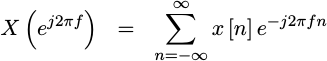
It is this third representation of the Fourier transform, known as the Discrete Fourier transform, that we’ll be discussing the implementation of today. I’m also going to argue that this is the only representation of the Fourier transform that can be numerically computed for any sampled finite sequence, but I’ll be glad to invite you to prove me wrong.
If you look at the form above, you can see it takes as input N data
samples, x[n],
and calculates one summation across those inputs for every value of k to
produce N
samples
out, X[k/N]. Given that there’s a complex multiplication
required for every term in that summation of N numbers, and that there are
N relevant outputs, this will cost N^2 painful multiplications to calculate.
If we just left things there, this transform, would be so hard to calculate that no one would ever use it.
Cooley and
Tukey,
however, described a way that the Discrete Fourier
transform
can be decomposed into two transforms, each of them being half the size of
the original, for the cost of only N multiplies. If you then repeat this
log_2(N) times, you’ll get to a one point transform, for a total cost of
N log_2(N) multiplies. At this cost point, the Discrete Fourier
transform
becomes relevant. Indeed, it becomes a significant and fundamental
DSP operation.
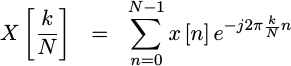
Let’s take a moment to scratch the surface of how this is done, using the “decimation in frequency” approach to decomposing the FFT that is used within this core. It involves first splitting the summation into two parts, one containing the low numbered terms and one containing the higher numbered terms.
 |
The left term captures the first half of the summation, whereas the right term captures the second half.
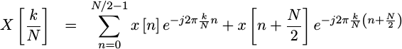
If you look at the two summation terms above, you’ll see that they share a
complex exponential,
e^{-j2pi kn/N}. We can factor this common term out to the right.
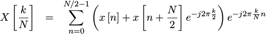 |
Once factored, this almost looks like the same summation we started with, only in a recursive form. The difference is that we are now calculating a smaller Discrete Fourier transform, summing over only half as many points as before. The big difference is a subtle modification to the inside.
To draw this out, let us consider even and odd frequency bins, 2k and 2k+1.
 |
We can simplify this further by the simple fact that e raised to any
integer multiple of 2pi will be one. Similarly, e raised to any odd
integer multiple of pi will be negative one. This allows just a touch more
simplification.
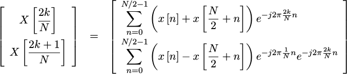 |
This means that with just a little bit of manipulation, we can split the calculation of one Discrete Fourier transform into the calculation of two similar Discrete Fourier transform, each that are only half the size of the original.
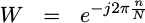
The frequency independent complex
number in the second line,
e^{-j 2pi n/N} is commonly known as a
twiddle factor. The generated
pipeline FFT will
use a lookup table to avoid the need to calculate this on the fly.
Reducing an FFT by
pairs of frequencies in this fashion is accomplished via what’s called a
butterfly. In the code
we’ll discuss below, we’ll use the term FFT
stage to reference
decomposing an FFT into
two smaller FFTs,
and we’ll call the calculation of the values within the parenthesis above
a butterfly.
I said I was going to gloss over the gory details, so I’ll start doing so here. These details are readily available to anyone who wishes to look them up.
However, there is one important detail associated with which
samples
the butterflies
are applied to that I don’t want to skip. From the equations above, you can
see that the butterfly
will be applied to
samples
n and n+N/2. What’s not so obvious is that we can then repeat
this same decomposition using
samples
n and n+N/4, and we can then repeat the decomposition again.
The other important detail in this process is that the result will be produced
in a bit-reversed
order. You can see some of that above. Notice how the values n and n+N/2
were used to calculate frequencies 2k and 2k+1.
Well come back to some of these details in a bit when we discuss how this core was verified.
Running the Core Generator
If you want to try out the core generator, you’ll need to download and build it first:
$ git clone https://github.com/ZipCPU/dblclockfft
$ make
I like to think that the project doesn’t have any dependencies. It would be more realistic to point out that it depends upon GCC (or other C compiler), binutils, make, and a basic Linux environment. (This is currently necessary for creating directories, etc.) The various bench tests currently require Verilator, though some require Octave as well, and the formal proofs of the various components require SymbiYosys and both the yices and boolector engines. Neither Verilator, Octave, nor SymbiYosys or the formal engines, are required to use the core generator, however. Feel free to correct me if there’s anything I’m missing here.
Once the “make” command completes, you
should have an fftgen program in the sw/ subdirectory within the core.
That’s what we’ll be working with.
Need an FFT? Let’s get started using this coregen!
Suppose you want a 128-pt FFT. You can simply run
$ ./fftgen -f 128This will create a directory fft-core, into which it will place the Verilog
code for this FFT, and
the various hex files for the twiddle
factors.
Of course, in any FPGA, bit size is closely related to logic usage within the core, and so it can be very important to control bit size. The example above will create an FFT with a default input bit-width of 16-bits per input. Not only that, but this width will grow at one bit for every two stages.
Would you rather have an FFT with a 12-bit input width?
$ ./fftgen -f 128 -n 12This will create a 128-pt FFT with 12-bit inputs and 16-bit outputs.
What if you only wanted a 12-bit output? You could limit the internal bit
growth, and hence the output size, to only 12-bits by adding -m 12 to your
command line.
$ ./fftgen -f 128 -n 12 -m 12By default, this will use twiddle factors (constant approximations of those complex exponentials) of 12-bits–the same size as the input bit width.
What if that’s not enough? An
FFT with
twiddle factors
the same width as the data will suffer from some amount of truncation
error. We can
increase the number of bits used by these twiddle
factors to help reduce this
truncation error.
Let’s increase them by making them two bits longer than the data at every stage.
To do this, we’ll add -x 2 to our command line.
$ ./fftgen -f 128 -n 12 -m 12 -x 2This will reduce the internal truncation
error associated with
calculating the FFT.
This truncation error
will decrease until about -x 4 or so, after which adding additional bits
bits is not likely to yield any significant additional improvements.
Voila! A wonderful FFT!
Well, not quite. The big problem with this FFT is that we’ve used hand-generated shift-add multiplication logic for many stages. These soft-multiplies are expensive, and may well consume all of the logic within your FPGA. If you are instead using an FPGA that provides hardware accelerated multiplies (i.e. DSP elements), then you can authorize the core to use some limited number of these DSP elements.
For example, let’s build an
FFT
using no more than 15
DSP by adding
-p 15 to our command line.
$ ./fftgen -f 128 -n 12 -m 12 -x 2 -p 15At this point, all of the multiplies within five of the seven stages of our 128-pt FFT will now use hardware multipliers, at three multiplies per stage. The last two stages don’t use any multiplies, since they can be accomplished simply using additions and subtractions.
On the other hand, if your signal will come into the core at no more than one sample every other clock cycle, then you can drop the number of multiplies used per stage from three down to two.
This is the -k parameter. -k 2 will cause the
FFT
to assume that you’ll never give it two
samples
on adjacent clocks.
$ ./fftgen -f 128 -n 12 -m 12 -x 2 -p 15 -k 2This will now use 2(N-2) multiplies for a 2^N point
FFT, of which
no more than 15 of these (-p 15) will use your
FPGA’s
DSP elements.
Need to use fewer
DSP elements?
Suppose no more than every third value required
a multiply? Then we could do -k 3, and use no more than one multiply per
stage.
$ ./fftgen -f 128 -n 12 -m 12 -x 2 -p 15 -k 3This could be very valuable when processing an audio signal, for example, that only ever has less than one sample every thousand clock ticks.
Other options of interest include -i to generate an inverse
FFT (conjugates the
twiddle factors),
-2 to generate an FFT
that can ingest two
samples
per clock, and so on.
Indeed, you can just run fftgen -h to get a list of all of the options this
FFT core generator will support.
$ ./fftgen -h
USAGE:	fftgen [-f <size>] [-d dir] [-c cbits] [-n nbits] [-m mxbits] [-s]
	-1	Build a normal FFT, running at one clock per complex sample, or
		(for a real FFT) at one clock per two real input samples.
	-a <hdrname>  Create a header of information describing the built-in
		parameters, useful for module-level testing with Verilator
	-c <cbits>	Causes all internal complex coefficients to be
		longer than the corresponding data bits, to help avoid
		coefficient truncation errors.  The default is 4 bits longer
		than the data bits.
	-d <dir>  Places all of the generated verilog files into <dir>.
		The default is a subdirectory of the current directory
		named fft-core.
	-f <size>  Sets the size of the FFT as the number of complex
		samples input to the transform.  (No default value, this is
		a required parameter.)
	-i	An inverse FFT, meaning that the coefficients are
		given by e^{ j 2 pi k/N n }.  The default is a forward FFT, with
		coefficients given by e^{ -j 2 pi k/N n }.
	-k #	Sets # clocks per sample, used to minimize multiplies.  Also
		sets one sample in per i_ce clock (opt -1)
	-m <mxbits>	Sets the maximum bit width that the FFT should ever
		produce.  Internal values greater than this value will be
		truncated to this value.  (The default value grows the input
		size by one bit for every two FFT stages.)
	-n <nbits>	Sets the bitwidth for values coming into the (i)FFT.
		The default is 16 bits input for each component of the two
		complex values into the FFT.
	-p <nmpy>  Sets the number of hardware multiplies (DSPs) to use, versus
		shift-add emulation.  The default is not to use any hardware
		multipliers.
	-s	Skip the final bit reversal stage.  This is useful in
		algorithms that need to apply a filter without needing to do
		bin shifting, as these algorithms can, with this option, just
		multiply by a bit reversed correlation sequence and then
		inverse FFT the (still bit reversed) result.  (You would need
		a decimation in time inverse to do this, which this program does
		not yet provide.)
	-S	Include the final bit reversal stage (default).
	-x <xtrabits>	Use this many extra bits internally, before any final
		rounding or truncation of the answer to the final number of
		bits.  The default is to use 0 extra bits internally.
$
I’ll admit this FFT generator project remains a bit of a work in progress, there’s just so much more I’d like to do! For example, it currently only calculates a complex FFT. There’s a real-to-complex stage that needs to be implemented in order to do real FFTs. I’d also like to implement a decimation in time algorithm, since having both will allow me to (optionally, under some pass-through implementations) remove the bit reversal stage. Eventually, I’d love to build a block processing FFT as well. All of these items are on my to-do list for this core, they just haven’t been done yet.
Still, it currently works as advertised. Care to try it?
Interfacing with the FFT Core
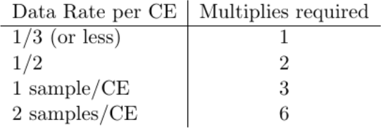
Once you’ve generated an FFT, it’s then time to try it out. To do that, you’ll need to connect it up to your design. The generated core has a couple of basic input ports, shown below and in Fig 3.
module fftmain(i_clk, i_reset, i_ce,
i_sample, o_result, o_sync); |
These basic ports are:
-
i_clkshould be self explanatory. This core consists of synchronous logic only, and everything is synchronous to the clock input. -
i_resetis a positive edge synchronous reset signal. If you would rather an asynchronous reset, there’s a-Aoption to generate logic using asynchronous negative edge resets. However, since I tend not to use them, I haven’t tested this option much. -
i_ceis a global CE signal. It is set to1on every clock where a valid new sample is available on the input. It’s very useful for processing signal that may be at a rate slower than the system clock, such as we discussed some time ago. Onceo_syncbecomes true, one data sample will come out of the core and be valid on every clock cycle thati_ceis high.If you use the
-k 2or-k 3options, you’ll need to guarantee thati_ceis never true twice in two samples or twice in three samples respectively, to allow the FFT a chance to compute the data.While this breaks the assumptions I described earlier for the global CE signal, specifically that nothing should act if
i_ceis false, doing so allows the FFT to share multiplication elements when possible.One final note here: if you want or need to control when the FFT starts processing, or specifically which sample is the first sample of the frame, you can use the
i_resetinput for that purpose. The first sample value wherei_ceis true andi_resetis false will be the first value into the FFT. -
i_sampleis actually a pair of values, both real and imaginary, stuffed into one signal bus. The real portion is placed in the upper bits, and the imaginary portion is placed in the lower or least significant bits. Both values are in traditional twos complement format, just stuffed together into a single input. -
o_resultis the output of one FFT bin from the FFT. It is in the exact same format asi_sample, save only that the output bit-widths used ino_resultmay be different from the input bit-widths used ini_sample.If you can’t remember what bitwidths the FFT was generated for, just check the
IWIDTH(input width) andOWIDTH(output width) local parameters in the main, or toplevel, FFT core file. -
o_syncis the last output in the port list. This signal will be true wheno_resultcontains the first output bin coming out of the FFT. This will be the zero frequency bin. Theo_syncsignal is provided to allow any following logic to synchronize to the FFT frame structure.The core does not produce an input synchronization signal to signal the first sample of the frame.
If the core is configured to handle two samples per clock, the data ports and port names are subtly adjusted. The new ports are:
 |
-
i_leftandi_rightreplacei_samplewhen/if you want an FFT that processes two samples per clock. They have the same format asi_sample. The difference is thati_leftis processed as though it came beforei_right. -
o_leftando_rightare the output values that replaceo_result. As with the two-sample per clock FFT inputs,i_leftandi_right,o_leftis the “first” output of the FFT ando_rightis the second one. Hence, if you include the bit reversal step theno_leftwill refer to an even output bin, ando_rightwill only ever carry information for odd output bins.
The particular core generated by fftgen is a
pipeline
FFT, rather than a
block FFT. This means
that the FFT is always
busy after accepting the first
sample.
Once the first o_sync is true, then
valid data is coming out of the
FFT. On every
sample
thereafter where i_ce is true, the
FFT
will produce another output
sample.
You may be familiar with another FFT implementation, that of a block FFT implementation. In a block FFT, a single block of samples would be provided to the FFT engine, after which the FFT engine would become busy and not accept any other samples. Once a block FFT finishes processing the samples given to it, then it becomes ready for a second block. As a result, a block FFT may have other external signals beyond the ones shown above.
The FFT implementation I am discussing today, however, is only a straight pipeline FFT.
Verifying an FFT
This blog remains dedicated to keeping students out of FPGA Hell. So, how did I make certain that this FFT implementation worked?
Let me begin by saying that “FPGA Hell” gains a new meaning when working with an FFT. FFTs are difficult to understand internally, particularly because it can be difficult to validate the data midway through. Yes, I’ve written multiple FFT implementations, both in software and now in hardware. Yes, I’ve gone through the mathematics. That doesn’t mean they are simple. Even with full access to every internal signal within an FFT they can still be a bear to debug. Indeed, I still get surprised at the end of this rather complex transform when signals suddenly pass through it properly.
Now that I’ve said all that, it should come as no surprise that debugging the FFT is really a story in itself. Let me try telling what I can of it.
When I first built the FFT, it was to support a GPS processing accelerator. I had a hard time limit that the FFT needed to meet, or the accelerated operation wouldn’t meet real time requirements. I became concerned during this process that the FFT wouldn’t be fast enough, so I built an FFT that could process two samples per clock.
To verify this initial FFT, I created test benches for all of the components. The test bench would work by running data through each component of the FFT. At the same time, I would double check the output values within the C++ driver of my various Verilator test benches. At first, the data was carefully chosen to find specific potential flaws within the various FFT components. Later tests then threw random data through the component(s) to prove their functionality.
Perhaps walking through an example might help explain this.
Initial Butterfly Verification
 |
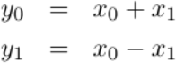
As an example of this initial functional verification method, let’s consider the implementation of the butterfly shown on the right. This should look familiar to you, as we discussed the equation for this earlier. It’s known as a “radix-2” decimation in frequency FFT butterfly, and it’s a primary component within the design. Indeed, the FFT is formed around calculating this operation repeatedly.
If we let
 |
Then we can represent this butterfly as,
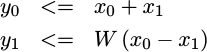 |
Where x0 and x1 are complex inputs to the butterfly, W is a complex
exponential constant coefficient, and y0 and y1 are complex outputs.
We can break this operation down further, and write
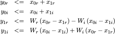 |
If this looks complicated while reading it, relax. It’s much more complicated in its actual implementation.
There are several problems with implementing this equation that aren’t immediately apparent from just reading it. The least of these problems are the four multiplies. Because multiplication is so expensive, I used a three multiply alternative in the actual implementation. But I digress.
Originally, the test bench would just create one line of text output per clock. This line would include the time step, then the inputs to the module, and finally the outputs from the module–all on the same line. Sometimes, I’d even place intermediate values on the line as well. The trick to making this work was to halt as soon as an invalid value was returned from the core, so that value could be examined. The disadvantage with this approach is that there are only so many values that can fit on a line that can be reasonably comprehended.
Eventually, I enabled VCD file generation as well, and then began examining output files via GTKWave in addition to the textual output.
To test the butterfly module, I provided initial inputs where all values but one were zero. I then provided inputs to this module where the coefficients were plus or minus one or plus or minus Pi.
To verify the proper functionality of the butterfly, I repeated the calculation within C++ inside my Verilator test bench. I then judged that, if the two matched, then the butterfly worked.
Once I tested all of the basic inputs outlined above, I then moved on to throwing random values at the butterfly to “prove” that it worked. In reality, this approach never “proved” anything, but it does help to provide some assurance. Eventually, I modified the butterfly test bench so that it would completely exhaust the entire space of possibilities. Be aware, though, such an exhaust can send massive amounts of text to your output stream, and fill up 42GB (or more) of VCD trace files.
The annoying problem with this approach to debugging is the sheer size of the data that needs to be searched through and processed once a bug is detected. A recent run, as an example, generated 42GB of VCD data. Ouch! That can be hard to process with GTKWave, and generating file size that large has been known to impact the user response time of my computer. I know I’ve wondered at times if my CPU needs to be given a hard reset, or just left to continue.
Still, this is a good example of how this FFT core was originally tested. Indeed, these bench tests remain within the repository. There are test benches for the regular butterflies, for the hardware assisted butterflies (those using DSPs), for the basic FFT radix-2 stages, the penultimate FFT stage and the final FFT stage. There’s also a test bench for the bit reversal stage and the FFT as a whole. These test benches still work, and they are available for inspection and test within the repository.
Making the FFT General Purpose
Recently, I came back to this FFT core generator to see if I could make turn it into a general purpose pipelined FFT, instead of one that could only operate in a two-sample per clock mode. Two big things changed in this process.
First, in hind sight, I realized many of the “special modules” of the
FFT
could be parameterized into a few simple Verilog modules. For example, the
2048 point radix-2 stage was fundamentally identical to the 64-point radix-2
stage with only a few differences that could be captured by parameters.
Likewise, the inverse
FFT
code was identical to the forward
FFT code, save
only that the twiddle factors
needed to be conjugated. In the end, only the top level component and the
coefficient files truly needed the core generator approach.
The second big change was that I wanted to support three versions of all of the butterflies, both the one using the soft multiplies and the one using the hard multiplies. I needed one version of each that would handle one operation per clock, one that would multiplex the three multiplies across two multiplication elements, and a third implementation that would multiplex the three multiplies across three multiplication elements.
There were other minor changes as well. For example, the bit reversal
stage
needed to be rewritten to handle one value per clock, as did the
final radix-2 stage of the
FFT. Further, the
core components had initially been written without setting the default_nettype
to none, and without using verilator -Wall.
As a result, the minor change of adding support for three types of single sample at a time streams turned into a major rewrite of the entire FFT.
That also meant that everything needed to be reverified. Test benches needed to be updated and … searching through GB of files for bugs that might or might not show up was becoming really annoying.
So, I switched to using formal methods to verify this FFT. Once I had proved that the simple modules of the FFT worked, there were only a few modules left. That’s when it became personal: would it be possible to formally verify the entire FFT?
Hold that thought.
For now, let’s walk through a quick discussion of how each section was verified.
Bit-Reversal
The bit reversal stage works by first writing a full FFT output into a piece of block RAM memory. When the second FFT output starts coming into the bit-reversal core, the core then switches to writing this new FFT into a second block RAM area. Then as more data comes in, the core ping-pongs between the two sections of memory.
Now, at the same time the bit reversal stage is writing incoming data into one memory area, it is also reading out from the other memory in a bit-reversed order.
 |
To formally verify the bit reversal stage, I let the formal tool pick an arbitrary address (and memory area) , and then applied the basic memory proof to that address. Further, any time a value is written into this special address, I assert that it wasn’t full before. When this special value is read out of the FFT, I also assert that the FFT is outputting the right value. In between, I assert that the memory contains my value of interest. It’s the same three basic properties we’ve already discussed, and it worked quite well in this context.
Last-Stage
 |
The last stage of the FFT is special. It implements the same radix-2 butterfly as any other stage, save that 1) it operates on adjacent pairs of data and 2) the complex exponential evaluates to either plus or minus one. That means all the work can be done using adds and subtracts–no multiplies are required.
 |
When I struggled to get this simple operation right, I groaned at having to build another test bench. I just wanted this thing to work and building and maintaining all those test benches were getting painful. Couldn’t I just prove that my code would work first using formal methods?
So I created a formal properties section in the laststage.v, and recorded a copy of the data that came into the core within that section.
	reg	signed	[IWIDTH-1:0]	f_piped_real	[0:3];
	reg	signed	[IWIDTH-1:0]	f_piped_imag	[0:3];
	always @(posedge i_clk)
	if (i_ce)
	begin
		f_piped_real[0] <= i_val[2*IWIDTH-1:IWIDTH];
		f_piped_imag[0] <= i_val[  IWIDTH-1:0];

		f_piped_real[1] <= f_piped_real[0];
		f_piped_imag[1] <= f_piped_imag[0];

		f_piped_real[2] <= f_piped_real[1];
		f_piped_imag[2] <= f_piped_imag[1];

		f_piped_real[3] <= f_piped_real[2];
		f_piped_imag[3] <= f_piped_imag[2];
	end
I could then verify that the data going out matched the known butterfly equations. First, there was the output that was the sum of the two inputs.
	always @(posedge i_clk)
	if ((f_state == 1'b1)&&(f_syncd))
	begin
		assert(o_r == f_piped_real[2] + f_piped_real[1]);
		assert(o_i == f_piped_imag[2] + f_piped_imag[1]);
	end
Then there was the output that was their difference.
	always @(posedge i_clk)
	if ((f_state == 1'b0)&&(f_syncd))
	begin
		assert(!o_sync);
		assert(o_r == f_piped_real[3] - f_piped_real[2]);
		assert(o_i == f_piped_imag[3] - f_piped_imag[2]);
	end
There are a couple important things to note here. First, I didn’t use
$past() to capture the incoming data. $past() works great for expressing
values for one (or more) clocks ago. The problem with this implementation
was the i_ce value. Were this value always 1'b1, or even always alternating
1'b1 and 1'b0, $past() might have been useful. However, I needed to make
certain that the formal proof properly checked whether i_ce was used
properly. That meant I had to allow the formal solver to pick when i_ce
was high and when it wasn’t. Hence, the output value, o_val = {o_r,o_i}
might depend upon $past(i_val,2), $past(i_val,3), $past(i_val,4),
or … you get the idea.
A little more logic was required to make certain I knew which of the two
values to output at any given time, y0 or y1, but no more logic than
that was required.
At this point, I started to get excited by the idea of formally verifying parts and pieces of this FFT. Assertions like this weren’t that hard, and they could be easily made.
So I moved on to the next module, the qtrstgae.v.
The Penultimate FFT Stage
I call the second to the last FFT stage the quarter
stage,
qtrstage. This is the stage that applies two radix-2 butterflies to pairs
within every set of four points. There were points 0 and 2, and points 1 and 3.
Like the laststage,
this stage
also required only additions and subtractions
to implement the necessary multiplies required by the butterfly. Unlike the
laststage, the
twiddle factors
in this penultimate stage required multiplication by 1, j, -1, or -j.
This can still be implemented with additions and subtractions–I just needed
to keep track of which values these additions and subtractions were applied to.
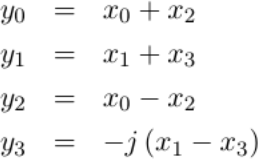 |
If you expand the last equation into its complex components, you’ll see that it truly can be represented by just additions and subtractions.
 |
For this stage, I tried the same basic proof approach as the prior stage. I created the sum and difference values, and verified that these indeed matched as they were supposed to. This logic was no more difficult than before. Aside from breaking the output into its real and imaginary portions,
	wire	signed [OWIDTH-1:0]	f_o_real, f_o_imag;
	assign			f_o_real = o_data[2*OWIDTH-1:OWIDTH];
	assign			f_o_imag = o_data[  OWIDTH-1:0];
I could then verify each of the various output real and imaginary values,
depending upon which state, f_state, the core was in.
	always @(posedge i_clk)
	if ((f_state == 2'b00)&&(f_syncd))
	begin
		assert(!o_sync);
		assert(f_o_real == f_piped_real[7] - f_piped_real[5]);
		assert(f_o_imag == f_piped_imag[7] - f_piped_imag[5]);
	end
These were the three easy proofs, bitreverse, laststage, and qtrstage.
How was I going to then prove the butterflies? Those depended upon a
multiply, and formal tools tend to really struggle with multiplies.
The Hardware Assisted Butterfly
|
This FFT core generator
uses two separate types of butterfly implementations.
The first
uses the DSP elements
within those
FPGAs
that have them. The core simply makes the assumption that A * B can
be implemented by the synthesizer in hardware. The second butterfly
implementation
uses a logic
multiply
implementation built specifically for this core.
Each of the two butterfly implementations has its own Verilog file, so we’ll
discuss them separately. In this section, we’ll discuss the hardware assisted
butterfly
that uses the DSP
elements.
When I started this major update, I had a working hardware assisted butterfly
implementation.
In that original implementation, everything moved forward anytime i_ce was
true, and it required three hardware assisted multiplication elements
(DSP blocks)
to complete.
However, if you are using an FPGA with only 90 DSPs that need to be shared between other operations (i.e. high speed filters), those DSPs can become very precious. How precious? When I built my first asynchronous sample rate converter, I quickly ran out of DSP elements before finishing. Were I to use an FFT in addition to such a poor design (it’s since been fixed), I might not have enough DSPs to make it work.
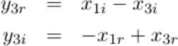
So I looked again at this algorithm to see if I could spare some multiplies.
What if the signal didn’t arrive at the rate of one sample every clock?
What if I could instead insist that the incoming data was less than half that
speed, so there would always be an idle cycle between any two clock periods
where i_ce was true? If that were the case, I could then share one
multiplication element between two of the three multiplies I needed to compute.
Alternatively, what if the signal didn’t arrive at a rate of every other clock, but would arrive no faster than every third clock? I might then share the hardware multiply between the three separate multiplies I needed to calculate.
You can see the possibilities in Fig 9 on the right.
 |
This required modifying my hardware butterfly implementation.
I managed to do this without too much fanfare, and without much work I modified my bench test and could get the hardware DSP to pass. I did the same for the regular (non-hardware assisted) butterfly as well. The problem was that the FFT kept failing in practice. It passed the component bench testing step, but yet still failed.
In frustration, I switched verification methods to formal.
I hadn’t wanted to do this at first. I am painfully aware that formal methods really struggle to handle multiplies, and these butterfly implementations both depended heavily upon the multiply. How could I test an algorithm that required multiplies, without running into this trouble?
The solution for me came from the formal methods concept of abstraction, something I have yet to discuss on this blog. (It’s a part of my formal methods class, and on my to do list for the blog.)
We’ll start with the basics. Here was the code I wanted to verify.
		always @(posedge i_clk)
		if (i_ce)
		begin
			// Third clock, pipeline = 3
			//   As desired, each of these lines infers a DSP48
			rp_one   <= p1c_in * p1d_in;
			rp_two   <= p2c_in * p2d_in;
			rp_three <= p3c_in * p3d_in;
		end
From processing the previous two modules, I knew how to set up a verification
test of the result: I’d copy the inputs into a memory delay line on every
i_ce, and then verify the result at the end given the incoming values.
I also knew that the hard multiply implementation “worked”. This was the one using the DSPs. Hence I didn’t need to verify that the multiply worked. Any tool that allowed me to do this was one where the multiply was supported and worked. I was willing to trust my tools.
I wasn’t willing to trust my own multiplication implementation–but we’ll come back to that in a moment.
So I replaced the hardware multiplies with something that was nearly equivalent, an abstraction. In this abstraction, the results were allowed to be any value, chosen by the tools, but meeting three criteria: 1) zero times anything is zero, 2) one times anything preserves the initial value, 3) negative one times anything negates the other operand, and 4) the same concept, but applied to higher powers of two instead of just one. This abstraction isn’t really a multiply, it just maintains some of the properties of multiplication.
You can examine it here in the abs_mpy.v
file
if you would like.
So, I replaced my multiplies with this abstraction. Here it is for the highest speed case where a data value could come in at any time.
	wire	signed	[((IWIDTH+1)+(CWIDTH)-1):0]	pre_rp_one, pre_rp_two;
	wire	signed	[((IWIDTH+2)+(CWIDTH+1)-1):0]	pre_rp_three;

	abs_mpy #(CWIDTH,IWIDTH+1,1'b1)
		onei(p1c_in, p1d_in, pre_rp_one);
	abs_mpy #(CWIDTH,IWIDTH+1,1'b1)
		twoi(p2c_in, p2d_in, pre_rp_two);
	abs_mpy #(CWIDTH+1,IWIDTH+2,1'b1)
		threei(p3c_in, p3d_in, pre_rp_three);

	always @(posedge i_clk)
	if (i_ce)
	begin
		rp_one   = pre_rp_one;
		rp_two   = pre_rp_two;
		rp_three = pre_rp_three;
	end
Then later, within the formal property section of the code, I allowed the formal tool to pick what data would come into the core and what coefficient (twiddle factor) would come in. I insisted upon my rules of multiplication with one and zero.
	always @(posedge i_clk)
	// Start by double checking that our delay line is valid,
	// similar to f_past_valid
	if (f_startup_counter > F_D)
	begin
		assert(left_sr == f_sumrx);
		assert(left_si == f_sumix);
		assert(aux_s == f_dlyaux[F_D]);

		if ((f_difr == 0)&&(f_difi == 0))
		begin
			assert(mpy_r == 0);
			assert(mpy_i == 0);
		end else if ((f_dlycoeff_r[F_D] == 0)
				&&(f_dlycoeff_i[F_D] == 0))
		begin
			assert(mpy_r == 0);
			assert(mpy_i == 0);
		end

		if ((f_dlycoeff_r[F_D] == 1)&&(f_dlycoeff_i[F_D] == 0))
		begin
			assert(mpy_r == f_difrx);
			assert(mpy_i == f_difix);
		end

		if ((f_dlycoeff_r[F_D] == 0)&&(f_dlycoeff_i[F_D] == 1))
		begin
			assert(mpy_r == -f_difix);
			assert(mpy_i ==  f_difrx);
		end

		if ((f_difr == 1)&&(f_difi == 0))
		begin
			assert(mpy_r == f_widecoeff_r);
			assert(mpy_i == f_widecoeff_i);
		end

		if ((f_difr == 0)&&(f_difi == 1))
		begin
			assert(mpy_r == -f_widecoeff_i);
			assert(mpy_i ==  f_widecoeff_r);
		end
	end
I found an amazing number of bugs in this fashion.
Even better, the proof completes.
The only problem was, at this point in my development, the FFT still didn’t work.
So I kept working.
The Soft Butterfly
The FFT has a second butterfly implementation, one that uses no hardware accelerated multiplies. Instead, it uses a (rather poor) multiplication implementation in logic. I say this implementation is rather poor simply because I haven’t yet optimized it, and because I know that better implementations exist. In my case, I wanted a single multiplication implementation that could be parameterized and yet apply to all bit-widths. Worse, that implementation needs to know what its own processing delay is. My bare-bones, basic implementation does all of the above, it just could be better. My own optimmized multiplication implementations doesn’t meet this criteria.
In the story of this FFT development, it was this part of the implementation that was most problematic for me. I didn’t dare replace the hand-built multiply within it with some abstraction, primarily because I didn’t trust it: I was always concerned there was a latent bug within the multiply. For example, what if I didn’t get the delay right?
This was also the stage that was responsible for several bugs that were a pain to chase down.
I ran bench tests
on this stage in all three modes: continuous i_ces,
one clock between i_ces, and two clocks between i_ces. When the design
failed, I adjusted each of these three elements to randomly include another
clock step with i_ce false. The tests would pass, and the design would fail.
The bug, as it turns out, was quite subtle.
Because the delay within my hand-made soft-multiply was dependent upon the bit width, and because this was captured by a parameter, and because the way I set up my Verilator tests only one parameter set was getting tested despite multiple parameters (and hence multiply delays) being used by the full FFT, the bench test might pass for one set of multiplication bit-widths and fail for the set that wasn’t bench tested.
I didn’t find this bug until I started using formal methods, although technically my formal methods approach suffers from the same problem of only testing some multiplication bit-widths.
For this soft
butterfly,
I call it butterfly.v, I created the same basic
properties I had been using for the hardware assisted
butterfly.
To my immense relief, this butterfly failed to pass formal methods (initially). Indeed, it failed very quickly. Why was this to my relief? Because I had been struggling to find the bug. It turns out, the bug was associated with the remainder of the multiplication delay divided by two or three–depending upon the mode. A subtly different timing implementation was required for each remainder, and I found that by using formal methods.
Yes, I could’ve found this using my test bench as well. I just had two problems when using it: First, I didn’t trust that it would try the right input combination to trigger the bug. Second, I was getting really tired of working through GB traces.
Now that I know what the problem was, the proof requires proving the FFT for multiple different potential parameter sets. SymbiYosys handles this nicely using tasks–something I haven’t discussed much on the blog. You can see the SymbiYosys script I used here, which includes the multiple task definitions if you are interested.
My problem with this proof is that while it quickly found my bugs in minutes, it struggled to prove that there are no bugs. By “struggled” I mean the took multiple days–so long that I never let it finish.
So I dug back into the proof. I set up criteria within every stage of the multiply to guide the proof: if multiplying by zero, the result in the middle should be zero, if by one, etc. I could then verify that the multiply would truly return zero on a zero input, or return the same value on a one input.
This still took forever.
The difficulty of this proof is also why this article took so long to write. I had the essential proofs working early on, but this one proof just seemed to take forever.
Part of the issue here is, how long are you willing to wait for a proof to return? I personally want my proofs to all return within about fifteen minutes. I’ll tolerate two to three hours, but not without grumping about it. However, this proof was taking over 72 hrs+ before I’d kill it. This is unacceptable.
 |
To understand the problem, consider Fig. 10. I had verified the long binary
multiply implementation, longbimpy.
I just wanted to prove some simple properties about the result, based upon the
initial values given to the
butterfly.
I wanted to verify that my estimate of the number of clocks
required by the long binary
multiply
matched the length of my FIFO. I wanted
to verify that the coefficients and inputs still matched the outputs, and that
one coefficient wasn’t getting confused with another piece of data.
To do this, I insisted that a zero coefficient must result in a zero result. A one coefficient must duplicate the data, and vice versa for the data. These are bare simple multiplication properties, but though they are simplistic they are sufficient for verifying if the right inputs are given to the multiplies, and if the matching results are drawn from them.
After about two weeks of running 48+ hrs proofs that I’d never allow to complete, I finally figured out how to bring the solution time down to something more reasonable. The trick? Asserting that the inputs to the multiply matched the butterflies copy of what those inputs were. This last assertion connected the proofs taking place within the multiply, with the proofs that were about to take place on the multiply’s outputs.
This necessitated a change to the portlist of the multiply, a change that only needs to be made for the formal proof and not otherwise.
module	longbimpy(i_clk, i_ce, i_a_unsorted, i_b_unsorted, o_r
`ifdef	FORMAL
	, f_past_a_unsorted, f_past_b_unsorted
`endif
		);
The unsorted post-fix above references the number of bits in the values i_a
and i_b. The algorithm internally sorts these two values so that the values
with the most bits is in i_b. The *_unsorted values just describe the
values before the bitwidth sort.
Then, internal to the butterfly itself, I assert that the f_past_a_unsorted
and f_past_b_unsorted values match the ones within the module. There’s a
bit of unwinding that needs to take effect, though, since the those values can
refer to any of the multiplies inputs depending upon the time step. That
places these values into fp_*_ic for the coefficient and fp_*_id for
the data.
The last step is to verify these two values match, for all three of the multiplication input sets.
	always @(*)
	if (f_startup_counter >= { 1'b0, F_D })
	begin
		assert(fp_one_ic == { f_dlycoeff_r[F_D-1][CWIDTH-1],
				f_dlycoeff_r[F_D-1][CWIDTH-1:0] });
		assert(fp_two_ic == { f_dlycoeff_i[F_D-1][CWIDTH-1],
				f_dlycoeff_i[F_D-1][CWIDTH-1:0] });
		assert(fp_one_id == { f_predifr[IWIDTH], f_predifr });
		assert(fp_two_id == { f_predifi[IWIDTH], f_predifi });
		assert(fp_three_ic == f_p3c_in);
		assert(fp_three_id == f_p3d_in);
	end
That assertion was sufficient to bring the proof time down from days to hours.
I can handle hours. I can’t handle days.
Full FFT Stages
 |
Because the butterflies were so hard to prove, I hadn’t spend much time trying to formally verify the separate FFT stages. I had just tested and verified that these worked using the traditional bench testing method–using carefully chosen and random inputs.
Then, later, I got to thinking: this FFT implementation is so close to having a full formal verification proof, why not just add this last piece to the set? So I dug into the FFT stage component.
In the language of this core generator, the FFT stage is that portion of the
core that accepts inputs and feeds a single radix-2 butterfly. This
means, for an N-point FFT stage, the core needs to read N/2 values into
memory, and then apply these values, the next N/2 input values, and a stored
ROM coefficient to the butterfly core. This butterfly core will return a pair
of values some number of clocks later. The data then need to be separated
again. One output value from the butterfly needs to go immediately to the
output, the other value must go into memory. Once N/2 values are output,
the butterfly becomes idle and the stored N/2 values can be returned.
Could this piece be formally verified?
Yes, it can. To do this, though, I replaced the butterfly implementation with a similar abstract implementation–like I had with the hardware multiply when verifying the DSP-enabled butterflies. This abstract butterfly implementation returned arbitrary values selected by the formal engine. It also had a multiplication delay within it that would be chosen by the formal engine, so that one proof could be made independent of the final butterfly implementation and multiplier delay.
Once done, the basic proof simply followed the three basic memory properties. That is, I allowed the formal engine to pick an arbitrary address to the input to the FFT stage, and then created a property to describe the inputs to the butterfly on the clock of this address.
	(* anyconst *)	reg	[LGSPAN:0]	f_addr;
	reg	[2*IWIDTH-1:0]			f_left, f_right;
	wire	[LGSPAN:0]			f_next_addr;
Any time the first value to the butterfly showed up and got placed into memory, I’d capture that value and assert that it remained in memory.
	always @(*)
		assume(f_addr[LGSPAN]==1'b0);

	always @(posedge i_clk)
	if ((i_ce)&&(iaddr[LGSPAN:0] == f_addr))
		f_left <= i_data;
I did the same on the second piece of data to enter the core.
always @(posedge i_clk)
if ((i_ce)&&(iaddr == { 1'b1, f_addr[LGSPAN-1:0]}))
	f_right <= i_data;
I then asserted that these values would be sent to the butterfly one
i_ce later.
wire	[LGSPAN:0]	f_last_addr = iaddr - 1'b1;

always @(posedge i_clk)
if ((i_ce)&&(!wait_for_sync)
		&&(f_last_addr == { 1'b1, f_addr[LGSPAN-1:0]}))
begin
	assert(ib_a == f_left);
	assert(ib_b == f_right);
	assert(ib_c == cmem[f_addr[LGSPAN-1:0]]);
end
Did you notice how I checked that the coefficient, ib_c, matched the ROM
memory, cmem, for this value? This is all the proof required for the
twiddle factor.
I then used roughly the same set of properties properties on the other side of the butterfly.
While I’d like to say that formally verifying this FFT stage helped me find some latent bug, that wasn’t the case this time. Once I debugged the FFT properties, this part of the core “just worked.”
The only thing was, I noticed that the block RAM read on the output path wasn’t optimized for all block RAM implementations. (Some internal RAM reads require the result be registered.) Because of the formal properties, when I changed this implementation to something more portable and better, I could make this change with confidence.
How much was verified?
I like to say that I have formally verified the entire FFT. You might even hear me boasting of this. This isn’t quite true. I only verified most of the FFT. (Queue the Princess Bride “mostly dead quote here …) I didn’t formally verify that the twiddle factors were right, that the soft multiply worked, or that the top level was properly wired together.
 |
To see how much was
formally verified, consider Fig 12 on the left. Everything
but the long binary multiply,
longbimpy,
and the toplevel,
fftmain,
has been formally
verified
I also only verified the components for particular parameter settings, not necessarily the settings used within the generated design.
The soft binary multiply, longbimpy, was functionally verified (i.e. verified by test bench), in an exhaustive sense. By that I mean that for a particular number of coefficient bits, I tested every single multiply input looking for problems. While this may be overkill, Verilator was fast enough to do this in less than a minute.
Conclusion
Does your design need an FFT? Please consider this core generator for that purpose. Using this core generator, you can create roughly any pipelined FFT implementation. Even better, because the core is completely open source, you can use this implementation within a Verilator simulation in a way you’d never be able to do with a proprietary FFT core generator.
The second point I’d like to draw from this FFT discussion is that, yes, SymbiYosys is up to an industrial formal verification task. It can be applied to very complex designs (no pun intended), piece by piece, just like we did with this FFT core generator.
You may also note that we didn’t formally verify the entire FFT at once. Neither did we formally verify that known input test vectors would produce known output vectors. If we did our job right, this will be a consequence. Somehow I just still didn’t trust the FFT until running known data signals through it. Hence, I still used simulation to ultimately verify that the FFT as a whole was working.
Finally, if you’ve checked out my FFT-Demo at all, you’ll see that an entire design using both co-simulated A/D, downsampling filter, FFT, and VGA output can all be simulated together. In that case, all of the components have been verified, but the full simulation of the entire design is still very valuable.
He that withholdeth corn, the people shall curse him: but blessing shall be upon the head of him that selleth it. (Prov 11:26)