
How to Debug a DSP algorithm
We’ve now written a linear upsampling algorithm, and discussed how to handle both bit growth and rounding within it. It’s now time to debug it, and prove that it does (or doesn’t) work.
The problem I’ve always had at this point is that my favorite tools don’t work very well for this task.
My favorite tool for debugging my own programs has always been (f)printf(). Sure, I’ve used gdb, and even its friendlier cousin ddd. It’s just that these two debuggers have not been my favorite tool. (f)printf() is still my favorite tool when it comes to debugging logic with Verilator. In the case of HDL, GTKWave comes in as a close second.
None of these approaches has ever worked well for me when debugging Digital Signal Processing (DSP) algorithms like this linear interpolator.
There’s just no substitute for the ability to plot waveforms, raw, processed, and even partially processed, on an ad-hoc basis. This ad-hoc capability is available through GNU’s Octave, Matlab, and to some extent with gnuplot. Of these three, my favorite has been Octave–mostly because I cannot afford Matlab.
In this post, we’ll return to examining our linear interpolator, but this time we’ll place it within a test harness to find out whether or not it works, and to see why or why not.
This test harness is the topic of this post.
Test Points
We know what we want our linear interpolator to do. That theory was well developed before we started. Hence, no validation is required. What we want to know instead is whether or not our linear interpolator is coming up with the right answers. That is, we want to verify that our Verilog logic works.
The easiest way to find any errors within our logic is going to be to build a duplicate set of logic to do the exact same thing, and then to compare the results to see if they match. While the approach isn’t perfect, the likelihood that both test fixture and system under test will be in error is much smaller than just the one being in error.
That means we are going to need to know:
-
The input(s) to our routine
-
Any intermediate results calculated by the routine, such as the slope the routine generated, and
-
The output of the routine.
The trick is that all of these values need to be lined up together in order for Octave to repeat the calculation and compare the result.
This isn’t quite as simple as it sounds, particularly because the outputs of
the linear
interpolator,
as we built it, aren’t evenly spaced every N ticks apart, but rather they get
produced in groups or bunches. Hence, when you look at them in
GTKWave, you may easily struggle to “see”
the waveform is that the interpolator is actually producing, as seen in Fig 1
below.
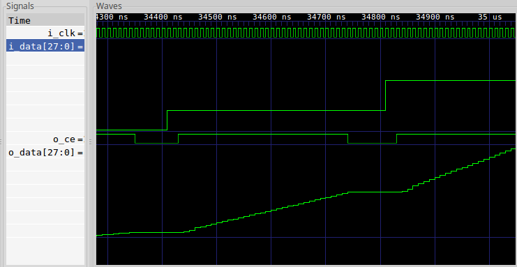 |
So, we’re going to add to our test harness a quick capability to write a debugging file out. We’ll write this file as a series of 32-bit integer binary values–something Octave will have no problems ingesting. For test purposes, we’ll also use some logic within the core to keep the test harness test points aligned.
Our goal will be to produce two data sets, using Octave, and to plot them one on top of the other. The first line on the graph will be our alternate calculation, done within Octave, showing what the linear interpolators result should be. The second line will plot what the result actually is. If the two functions lie on top of each other, then we’ll know our algorithm works.
The Test Harness
Let’s look through how the test harness for this linear interpolator is put together. While in many ways it’s just like any other Verilator based test harness, one thing that makes it very unique is what happens after the clock tick. To keep this simple, we’ll work in broad brush strokes to explain how this works, skipping large portions of it. If this gets confusing, please look back at our first Verilator tutorial, or even the test harness itself to see what’s going on.
To set this up, at the beginning of the test harness’s main routine, I created a debugging output file and pointer:
const   char    *DBGFNAME = "dbgfp.32t";
FILE    *dbg_fp;

dbg_fp = fopen(DBGFNAME,"w");
This file will also need to get closed when we’re all done.
Second, it turns out that picking the right interpolation frequency is rather important. You want your input clock to be fairly low, and your output clock fairly high if you want to make the pretty looking pictures below. Testing with an output clock rate very near the input clock rate can also be very useful and instructive as well, it just tends to be harder to understand the results.
For this test harness, I set the input sample rate to be one input sample for every forty clock ticks.
unsigned iclocks = 40;Third, we need to pick a signal to evaluate. I chose a sine wave. I set this to be at a fairly low frequency, 24 input samples per wavelength, because it will help to reveal any problems with our interpolator. Higher frequencies may also help, but they’ll test and reveal a different set of errors.
The sine wave function call takes place between one input sample and the next.
To create the desired frequency, we’ll step the phase forward by some angle
on every input sample. In the test
harness
code snippet below, I have called this step dphase, for a phase difference
or phase step.
// dphase is the phase increment of our test sinewave.  It's really
// represented by a phase step, rater than a frequency.  The phase
// step is how many radians to advance on each SYSTEM clock pulse
// (not input sample pulse).  This difference just makes things
// easier to track later.

// double	dphase = 1 / (double)iclocks / 260.0, dtheta = 0.0;
double	dphase = 1 / (double)iclocks / 24.0, dtheta = 0.0;
printf("DPHASE = %f\n", dphase);

while(...) {
	...

	// As well as the phase of the simulated input sinewave
	dtheta = dtheta + dphase;
	if (dtheta > 1.0)
		dtheta -= 1.0;

	// Do I need to produce a new input sample to be interpolated?
	if (inow >= iclocks) {
		...
		// Calculate a new test sample via a sine wave
		rv = cos(2.0 * M_PI * dtheta);
		...
	}
	...
}
Notice how dphase increments the actual phase, dtheta (double valued
theta). Further, any time dtheta wraps, we just subtract one to keep it
between zero and one. Then, when an input sample is required, we use this
phase as an input to the cosine function.
Fourth, there’s no reason to run this simulation until your PC needs to be rebooted. Hence, we’ll only look at a finite number of clock ticks before halting our simulation:
while(clocks < MAXTICKS) {
	clocks++;
	...
}
Finally, the real important part of any DSP debugger, in Verilator (or any C++ algorithm for that matter), is to output values that you can then ingest into Octave.
For our example, we’ll pick the inputs and outputs of the linear interpolator, together with four internal values. These will all be converted to signed 32-bit integers, and dumped to a file: six outputs at a time.
// If the core is producing an output, then let's examine
// what went into it, and what it's calculations were.
if (tb.o_ce) {
	// We'll record six values
	int	vals[6];

	// Capture, from the core, the values to send to
	// our binary debugging file
	vals[0] = tb.i_data;
	vals[1] = tb.o_data;
	vals[2] = tb.o_last;
	vals[3] = tb.o_next;
	vals[4] = tb.o_slope;
	vals[5] = tb.o_offset;

	// Sign extend these values first
	...

	// Write these to the debugging file
	fwrite(vals, sizeof(int), 6, dbg_fp);

	// Just to prove we are doing something useful, print
	// results out.  These tend to be incomprehensible to
	// me in general, but I like seeing them because they
	// convince me that something's going on.
	printf("%8.2f: %08x, %08x, (%08x, %08x)\n",
		rv, tb.i_data, tb.o_data, vals[0], vals[1]);
}
You’ll see in the next section, when we discuss the Octave test script, why we chose a constant number of values, and a common type for all of these same values.
The Octave Script
The first step to processing this data within Octave is to load the information into Octave. You’ll notice that all of the data we produced was uniform in type, and all of the records had the same number of samples, six. This makes loading the file into octave very easy. Indeed, it’s so easy that I usually do it by hand for the first several rounds of debugging, before I turn it into a script:
fid = fopen('dbgfp.32t','r');
dat = fread(fid,[ 6 inf] ,'int32');
fclose(fid);

% Assign names to these values
i_data  = dat(1,:);
o_data  = dat(2,:);
o_last  = dat(3,:);
o_next  = dat(4,:);
o_slope = dat(5,:);
o_offset= dat(6,:);

% We used 28 bits for our values internal to our simulation.  We'd like to
% plot our sine wave here between +1 and -2.  Hence, we'll need to scale
% them by 1/2^27.
nbits = 28;
mxv = 2^(nbits-1);
I think if I needed multiple data types, I’d probably first promote values to the largest type, and if that didn’t work I’d create multiple data files.
Now that our data has been ingested into Octave, let’s see if we can redo the arithmetic the FPGA is supposed to do, only this time in double precision math.
In this case, all the required math was discussed in our first post, so here we just repeat it.
redo = o_last + ((o_next-o_last).*o_offset)/mxv/2;
redo = redo / mxv;
One key difference in this version, from the discussion of how to do this
within the FPGA, is the divide by mxv*2. This comes back to a bit growth
issue, but a fixed vs floating point version of it. o_offset, as you may
recall,
is an integer being used to represent a value between zero and one.
Hence, we need to divide it by its scale factor to turn it back into a floating
point value between zero and one.
We’re also dividing our result, and indeed our input values as well, by mxv
so that we can plot the result between more reasonable bounds.
All that remains is to plot the results and see how well (or poorly) we did.
plot(t,i_data/mxv,'b;Input Signal;',
	t,redo,'r;Octave results;',
	t,o_data/mxv,'g;Interpolated/Output Signal;');
axis([2501,3000,-1,1]); grid on;
title('Comparing output results to Octave calculated results');
xlabel('Output Samples');
ylabel('Units');
Plotting data like this will really help you see problems in your code, and by seeing them, recognizing them will become easier to do.
Bugs I found
I really dislike sharing buggy code on this Blog. Sorry. As a result, I’m not going to show how how I messed this up along the way. (My code always works the first time, right?) Therefore, if you examine the linear interpolation example Verilog code, you’re not likely to find any bugs within it. (I won’t put it past you, though–as of today, I’ve only bench tested this component.)
In reality, there were bugs within it when I first simulated it.
-
The first bug I struggled with was a bit-width bug.
At several points during the linear interpolation algorithm, bits need to be selected and even dropped.
When I first ran this test, I dropped some of the more significant bits along the way. The result looked very jumbled. Further, since I was trying to view a sinewave in GTKWave, they looked even more jumbled. If you think you are struggling with this problem at all, try increasing the bit width (there’s a reason it’s set to 28 for this test), and backing away from full range to see if it helps.
Because the number of input bits in our test is so large, this problem can be see to have a clear signature (now) in Fig 2.
Fig 2: Internal bit selects in error 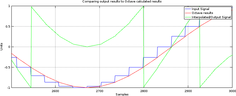
Once the algorithm works, you can remove any extra bits that were needed to test and prove it.
-
Signed multiplies are different from unsigned multiplies
This was another of my problems.
If you aren’t familiar with this problem, the consider multiplying some two’s complement 3’bit numbers together. A
-2would be represented as3'b110. Multiplying-2times-2should be a six bit-4, or6'b111100(Remember to add the bit widths of the inputs together to get the final bitwidth.) However, if you use unsigned multiplication then3'b110(6) times3'b110(6) is 6’b100100 (36) not 6’b111100. See the difference?You’ll notice this problem when everything works properly for positive numbers, and then fails for negative numbers. Indeed, if you ever see a result where things work in sections but not entirely, then you might want to check for this bug.
Fig 3: Unsigned vs Signed Multiplication Error 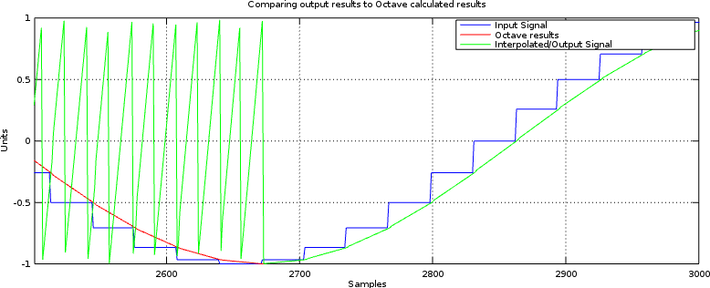
To fix this, I needed to declare the inputs to the multiply to be
signedwire’s or registers. I also needed to extend the unsigned time offset by a zero bit, to make sure it had the right sign. Once done, this bug cleared up as well.
You can find the final working linear interpolator here. The two bugs listed above have been fixed. As a result, the interpolator’s test bench output now looks like Fig 4 below.
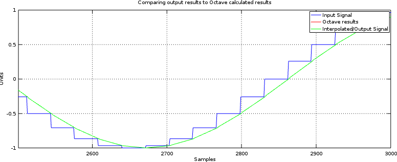 |
Not bad, huh? In fact, it’s just the result we wanted.
When Simulation doesn’t Match Realtiy
Since I’ve only tested this linear interpolation core under simulation, there may well be some residual problems if/when I try it on some actual hardware. It’s just a fact of life.
If you ever find yourself in that situation, then just repeat the same test, or one similar, but this time do it within the hardware itself. Remember, that was what your internal scope was for, right?
You can also use the debugging method discussed here, should you have problems where this works in simulation but not in hardware. Further, feel free to post any bugs below, or on the issues page for the GitHub repo, and I’ll fix anything you point out.
Lessons Learned
This example should illustrate for you two important lessons:
-
To determine if an FPGA algorithm is working, create another (similar) non-FPGA algorithm and test the two against each other.
In this example, we compared an Octave script’s version of our interpolator (we called this
redo) with the outputs of our Verilog interpolator. When they matched, as in Fig 4 above, we knew the algorithm worked.While this example accomplishes our needs for debugging a DSP algorithm, the same approach can (in general) be applied to many other FPGA algorithms. For example, you can find my UART protocol validator here, my QSPI flash validator here, and an SD-Card SPI-based protocol validator here.
-
The easiest way of writing the logic twice with a DSP algorithm is to do (and plot) the work within Octave.
The neat thing about Octave is that you can plot various things in an ad-hoc manner. Data can be scaled, reshaped and resampled, Fourier transforms may be applied, axes can be changed, labels adjusted, screen sizes changed, bit widths adjusted, etc., all very quickly and easily.
As an interesting side note, I once debugged the signal processing internal to a two-way radio communications channel in a similar fashion to this. This approach really works very well.
Feel free to share your own experiences below!
This they said, tempting him, that they might have to accuse him. But Jesus stooped down, and with his finger wrote on the ground, as though he heard them not. (John 8:6)