Understanding the effects of Quantization

Some time ago, I described on this blog how to use a CORDIC algorithm to rotate x,y vectors by an arbitrary angle and how to build a rectangular to polar conversion using the same basic methods. What I didn’t post was a test bench for those two routines. As a result, the presentations are really incomplete. While I have declared that they work, I have not proven that they work. Neither have I demonstrated how well they work.

What makes matters even more difficult is that proving that a (core generated) CORDIC algorithm works is not trivial. While generating a straight-forward test bench may be simple for one set of CORDIC parameters, the same test bench may not work for all parameters. In particular, the arbitrary parameters of input, phase, internal accumulator, and output bit widths are all going to have an affect on the performance of the overall CORDIC algorithm. How shall we understand how well this algorithm works for any particular set of parameters?

To answer these questions, let’s examine quantization effects. We’ll start by reviewing the definitions of some probabilistic quantities: the mean, variance, and standard deviation. We’ll then examine quantization noise according to these properties. Using these results, we can then draw some very general rules of thumb that we can then use in a later post to build a test bench for our CORDIC algorithm. Indeed, the results presented below will be generic enough that we may apply them to many other algorithms as well.

Some quick statistics

Understanding quantization effects requires a very basic understanding of probability. Probability involves the study of random variables, and how they behave.

In the study of probability, random variables are characterized by their probability distribution. A probability distribution is basically a function that can be used to define the probability that a random variable attains a particular value. The two requirements on a probability distribution function are first that all of the elements are non-negative, and second that the sum of all of the elements must be one.

There are two basic types of probability functions: probability mass functions (PMF) and probability density functions (PDF).

For random variables drawn from a discrete set of values, the probability distribution is described by a PMF. The PMF describes the probability of a random variables equalling a specific value from a discrete set.

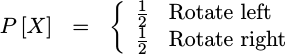
One discrete set that will interest us within the CORDIC algorithm is the set of two possibilities, each of which may be selected with equal probability.

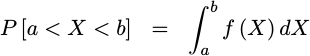
The other type of probability function describes a continuous random variable. This is the type we shall focus on today. Continuous probability distributions are defined by a probability density function (PDF). Unlike the PMF discussed above, PDFs are used to determine whether or not a random number falls within a range of values, as in:

These two functions, whether the PMF or the PDF as appropriate, completely characterize how a random variable is selected from among the possible values it may obtain.

Now that we can describe a random variable, the next step is to draw some conclusions from it. To keep things simple, we’ll examine three functions of a random variable. The first is the expected value. From there, we can define the mean, variance, and even the standard deviation.

The expected value of a random variable is defined as the sum, taken over all values the variable might assume, of the product of the probability of the variable taking on that value and whatever the expectation function is. While that sounds pretty confusing, the equation itself for an expected value is simpler than the description I just gave. For a continuous probability distribution over the real number system the expectation is defined by,

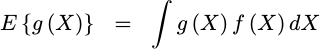where X is our random variable, g(X) is an arbitrary function of the random variable, X, f(X) is the PDF associated with this random variable, and the integral is taken over all real numbers. We’ll use this expression to define the expected value of a function, g(X), which we’ll then note as E{g(X)}.

Even this appears more complicated than it need be, since in our discussions below we’ll let g(X) be simple things such as X, X^2 or even the sum of two random variables, X+Y. We’re also going to let f(X) be something as simple as the constant 1 between -1/2 and 1/2, and zero other wise. In other words, don’t let the formula scare you: it’s easier than it looks.

Further, because the PDF is unitless, the units of the expected value are the same as the units of g(X). Hence, if g(X) is X^2, and X is a voltage, then the units would be voltage squared.

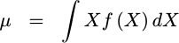
From this definition of the expectation we can now define the mean. The mean is defined as the expected value of the random variable itself, E{X}. We’ll use the Greek character mu to represent it, sometimes noting it as a u. If we just use the equation for expectation presented above, then this mean is calculated from,

You may be familiar with the statistical process of averaging. a set of measured values in order to estimate a mean. This is subtly different from the definition of the mean of a probability distribution that we just presented above. In the case of the statistical mean, a set of samples are drawn from a random distribution, and then averaged. The result of this method is a new random variable, which is often used to infer information about the probability distribution of the set of random variables from which the statistical mean was computed. The mean defined above, however, is completely characterized by the (assumed known) probability distribution of the random variable in question.

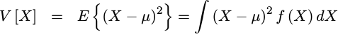
The next useful quantity we will be interested in is the variance of a random number. This is defined by the expected value of the random variable, minus its mean, squared. We’ll represent this value with a V[X], to note that it is the variance of the random value X.

We’ll use this definition of the variance later to analyze the errors within our CORDIC calculation.

The third useful quantity is the standard deviation. The standard deviation is defined by the square root of the variance. We’ll use the Greek letter sigma to represent this quantity.

Perhaps you noticed above that the units of variance were the units of X squared. (f(X) has no units) The reason why we even need a standard deviation at all is so that we can have a value that represents the spread of a random variable, but with the same units as X. This will make it easier to talk about and reason about the variance, even though the standard deviation measure itself doesn’t fundamentally offer any new information beyond what is already contained within the variance.

The above discussion may well be the shortest discussion of probability you will ever come across. As such, it’s rather incomplete. I would encourage anyone interested to either read the wikipedia articles cited above, or to take courses in both probability and statistics to learn more. It’s a fun field.

For now, we now have the basics of what we need to examine quantization effects.

Quantization Noise

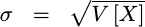
Quantization is the process that takes a continuous value and representing that value by a single value from a discrete set. Electrically, perhaps the most classic example of quantization is an analog to digital converter (ADC). Such a converter takes an input voltage, which may best be represented as a continuous value, and turns it into one of a number of discrete values. Fig 1 below shows an example of this.

Fig 1: Converting a continuous waveform into discrete values

In this example, the blue sinewave was the original value, and the discontinuous red lines represent a set of discrete values that each of the voltages within the sinewave were mapped on to.

ADCs also sample signals. Sampled signals are also discrete in time, and not just in value. For our purposes in this post, we’ll postpone the study of sampling for later, and just focus on the quantization effects.

Fig 2: An example quantization function

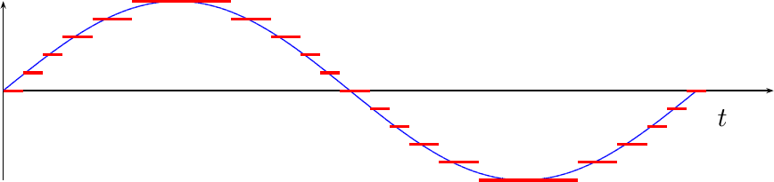
In general, the quantizater within an ADC may be considered to be a function with a continuous input, x, and a discrete output, y. One such function is shown in Fig 2 at right. A well built ADC will have evenly spaced discrete sample samples, y, and it will map all voltages, x, to their nearest sample value, y. What this means is that the difference between a sample value and the value it represents, y-x, will always be half the distance between samples or less.

Of course, quantizing any signal will distort the signal. This is easily seen by the simple fact that the red and blue lines in Fig 1 above are different. The desired value was shown in blue, the reality at the output of the ADC is shown in red. It is the difference between the two signals forms the topic of our discussion below.

Let’s define the difference between the original voltage and its quantized representation quantization error. As an example, the quantization error associated with Fig 1 above is shown below in dark green in Fig 3 below.

Fig 3: Quantization error, shown in green

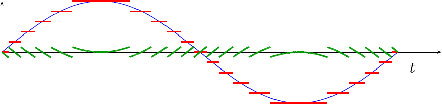This means that we can consider any received waveform to be the sum of two signals. The first is the signal of interest, shown in blue above. The second is the quantization error signal shown in green in Fig 3.

Our goal will be to understand the statistics of this quantization error.

To analyze this error, we’ll first notice that for a single sample, the difference between the analog voltage and the ADC result lies between -1/2 and 1/2 of a quantization level. In Fig 3 above, there are two thin lines running horizontally at -1/2 and 1/2. These lines illustrate the bounds of this error.

We’re going to treat this error as a random variable and assume that all of these differences are both independent and identically distributed. As one final assumption, we’ll assume that these quantization errors are uniformly distributed between -1/2 and 1/2, with the same units as our sampled values have. (You could do this in units of Voltage, it’s just a touch more complex.)

That gives us our PDF,

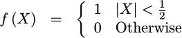and allows us to characterize our quantization “noise”. It also greatly simplifies any math we’ll need to do in order to calculate expectations, since we can now drop the f(X) function and then only need to integrate from -1/2 to 1/2.

For example, using this PDF, we can now prove that the mean of this error is zero.

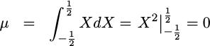In many ways, though, this proof is backwards. If all you did was to look at Fig 3 above, you could visually see that the mean of any quantization error should be zero. The amount of time the green line is above zero can be seen to be equal to the amount of time it spends below zero. Therefore, this mathematical proof really only (partially) validates our choice of distribution, rather than telling us anything new about our error.

A zero mean distribution will make our variance calculation simpler, since we no longer need to the mean as part of the calculation. With a zero mean, we now have

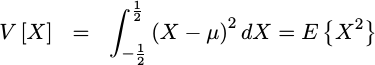for our variance. In other words, the variance of this quantization noise is simply given by the expected value of X^2.

We can now evaluate the integral, and quantify the variance of any quantization error:

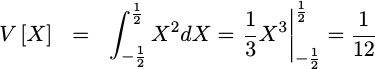If you look at the units of this variance, you’ll notice that they are the units of X squared. (f(X) and dX are unitless.) For this reason, it doesn’t make sense to compare values of X against this variance at all. For example, to ask whether or not the results of the CORDIC are within some number of variances from the right answer would involve a units mismatch. The standard deviation, however, captures this same information while maintaining the same units that X had. Since it’s just the square root of the variance, the standard deviation of any quantization error is simply the square root of 1/12 or equivalently

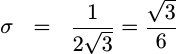Although this is the “proper” mathematical form for this standard deviation, I still tend to think of it as the square root of one over twelve.

These results, both for the variance and the standard deviation of quantization error, are the fundamental results of this section. We’re going to need these results as we try to calculate the errors we might expect from a CORDIC–or any other DSP algorithm for that matter. First, though, let’s look at what happens to this quantization and its variance when we apply a mathematical algorithm to our signal–such as we will within the CORDIC.

Rules for thumb

Two rules of thumb will help us facilitate using the variance of the quantization error to estimate algorithmic performance. These two rules regard how multiplying by a constant affects the variance, as well as how adding two random values together affects the variance.

The first rule deals with multiplying a random variable by a constant number. This operation increases the variance in the random variable by the square of the constant. This follows from the definition of variance:

For our second rule, we’d like to add two random variables together. We’ll insist on two assumptions. The first is that the two random variables are continuous and independently distributed, and the second is that they both have zero mean. From there, let’s look at the variance of the sum of two random variables.

The proof of our property is a touch more complex than the last one since any time you have two random variables you have to deal with a joint distribution. In general, the joint distributions is a bi-variate PDF, such as f(X,Y). Further, the single integral now becomes a double integral over both X and Y. However, since we assumed that these two random variables would be independent, their combined distribution can be expressed as a product of the distribution for X, f(X), and the distribution for Y, g(Y). g(Y) in this case is a different function from the g(X) above, since in this case it is the distribution function for the random variable Y. We’ll still need to integrate over both X and Y, but this simplification will help us split the double integral into two separate single integrals.

Now that we have our terms, we can now develop an expression for the variance of the sum of two random variables:

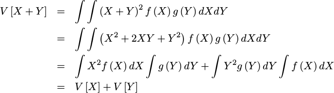In sum, the variance of the sum of two independent random variables, such as the X and Y above, is the sum of their individual variances.

Just for completeness then, here are the two properties we’ll need later.

The first property is how scale affects variance:

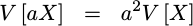To generate this property, we assumed that the random variable had zero mean. The property actually holds of random variables with non-zero means as well, but I’ll leave that as an exercise for the student.

The second property was the variance of the sum of two random numbers:

This property was dependent upon the assumptions of zero mean, and independent distributions. However, as with the first property, the zero mean assumption only simplified our proof–it wasn’t required.

Using these two properties, we can now return to our CORDIC algorithm(s) and consider the question of whether or not the algorithm(s) even work.

Coming up

As we look forward to future posts, I’ll try to keep those discussions simpler. I apologize for depth of this discussion, but if you want to prove how good an algorithm such as the CORDIC algorithm is, you are going to need some of this math. (If you know another way, let me know.) From here on out, I’m going to try to just use these results rather than rehashing today’s lessons.

If you found these lessons informative, then that’s wonderful! If you’ve never heard any of this before and it actually makes sense today, then I’m flattered. The concepts aren’t necessarily that simple.

On the other hand, if you are not familiar with the study of probability at all, then you may have found that the proofs and discussions above, regarding probability distributions and quantization error, read like a foreign language. If you feel like that is you, then let me commend to you the study of probability. I found the coursework to be a lot of fun, and enjoyed the study myself.

This lesson, though, sets us up to build the test bench that we need to put together for our CORDIC algorithm. Once we have proven the CORDIC’s capabilities, we can then turn around and use it to create a generic filtering test bench. With a generic filtering test bench, we can then build and test several digital filtering approaches that can be used within an FPGA.

If the Lord wills, then that’s where we’ll go next.