
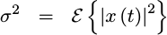
Cheap Spectral Estimation
If you have to debug a DSP algorithm, there are a couple of tools available to you. We’ve already discussed grabbing data samples and calculating histograms. We’ve also discussed taking FFTs of your data. But what if you want to estimate the spectral content of a signal within your FPGA on a platform that doesn’t have the resources to accomplish a full FFT?
 |
Certainly an
FFT
is the ideal operation to estimate spectral content: window
a segment of an incoming signal,
perform an FFT
on that segment and then magnitude square each of the output
samples for
visual effect. Is the result too “noisy”? If so, you can average several
FFTs together so that
you can “see” the spectral shape of what’s going on in your environment.
It’s just that all this comes at a cost. In my own pipelined FFT
implementation, each stage
requires between one and six multiplies together with enough block RAM to
hold an FFT.
At log_2(N) stages per
FFT, this resource
requirement
can start to add up.
On the other hand, what if I told you that you could get (roughly) the same spectrum estimate for only the cost of a single DSP element, about two FFT’s worth of block RAM and some LUTs to control the whole logic? Well, that and a nearby CPU?
How about if I do one better, and say that the algorithm is easier to debug than an FFT? (FFT internals are notoriously painful to debug.)
There’s no real trick up my sleeve here, nothing more than plain old good engineering practice: if resources are tight in one location, such as in an iCE40 FPGA SDR application, you just move the resources you need to another location where they aren’t nearly as tight.
Let’s take a peek today at how we can move the spectral estimation problem from the FPGA to a nearby CPU without sacrificing (much) of the FFT’s capability.
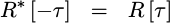
The key: Wiener-Khinchin Theorem
The key trick to this whole exchange is the Wiener-Khinchin theorem. The Wiener-Khinchin theorem states that the Fourier transform of the autocorrelation function is equivalent to the Power Spectral Density function. Using this principle, we can estimate the autocorrelation of a signal and then later take an FFT of the autocorrelation to get our Power Spectral Density estimate.
Let me back up, though, and start out closer to the beginning. Imagine you are in a lab and you have a signal you want to analyze. Perhaps you want to verify the shape of a low-noise amplifier, or find out whether or not there’s any interference from your digital electronics into some analog band, whether the signal you are transmitting from across the room made it into the receiver, or for that matter why your algorithm isn’t working no matter what it is. What would you do? You would place your signal into a spectrum analyzer and examine it’s content by frequency on the screen.
 |
The modern day digital spectrum analyzer will take a snapshot of that signal, possibly window the snapshot somehow, and then plot the Fourier transform of the result on the front panel. Mathematically, this operation looks somewhat like,
 |
where x(t) is the received waveform you wish to examine, h(t) is any
potential
window
function, T is the length of the observed
window, t_o is the middle of
the snapshot window and 1/T is the spectral resolution you have requested on
the front panel. The device
then plots this |X(t_o, f)|^2 value against an f/T horizontal axis.
At this point, I would typically look at the screen and convince myself the
spectral estimate is too “noisy” to do anything with, and so I’ll up the
number of averages. Let’s try N averages.
 |
Here, the plot settles out quite nicely and you have a reasonably good estimate of what the spectrum of your incoming signal looks like.
What we’ve just done is to estimate the Power Spectral Density of our incoming waveform.
The Power Spectral Density is defined as the expected value of the FFT of your signal, magnitude squared, as the size of the FFT grows without bound.
 |
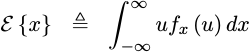
For those who aren’t familiar with probability and statistics, an expected
value
is just an average. For those who are, please forgive my heresy, I just
misspoke. An expected value
has a very specific mathematical definition that depends upon the probability
density function of the underlying random value. Specifically, the expected
value of something, noted below as E{x} for the expected value of x,
is defined as the integral of that something times the power spectral density
of the random variable, shown below as f_x(u), across its range, shown
below by the infinite limits of the integral.
 |
Taking “averages” only estimates the true mathematical and underlying expected value–a difference which will come back to haunt us when we try to test today’s solution.
If you are willing to bear with me for a little math, let’s see if we can simplify this expression for the PSD into something more useful. The first step to doing so would be to expand out the conjugate squaring operation that takes the absolute value squared of the FFT within. Unfortunately, this will leave us with a nasty double integral.
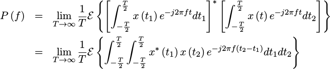 |
At this point, we can move the
expected value
inside the integrals and replace the
x^{*}(t_1)x(t_2) expression with the
autocorrelation
function of our signal. This will require a change of variables in a moment.
For now, let’s define the autocorrelation function of a signal as the expected value of our signal multiplied by itself at some offset.
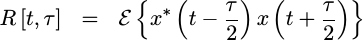 |
You may note that I’ve chosen to place t between the two points that are
multiplied together. This follows from
Gardner’s work on
cyclostationary signal
processing,
although we’ll adjust things back to the more familiar form next.
In particular, if our signal is wide sense stationary
(WSS), this function will
be independent of time. That means we can remove the time dependence of the
autocorrelation and just
represent it as a function of time difference, or tau which is also called
the “lag”.
 |
(As a side note, I’ll just point out that no observed signal has truly been
WSS, but the approximation
tends to simplify the math. As I mentioned above, I personally find a lot of
meaning in cyclostationary
signals, where
R[t,tau] isn’t independent of t but is rather periodic in t, but even
that approximation has its limits.)
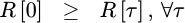
This autocorrelation has
some useful properties to it which we’ll come back to in a bit in order to
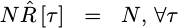
debug our own algorithm. For example, R[0] will be greater than all other
![`R[tau]`](/img/cheapspectra/eqn-Rtau.png) values.
values.
 |
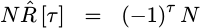
Similarly, the autocorrelation function can easily be proven to be conjugate symmetric in time.
 |
This will allow us in a moment to only estimate half of the function, and yet still get the other half for free.
So let’s bring the
expectation inside the
integral of our
PSD
expression, and then replace the
expectation
of x(t_1)x(t_2) with this new
expression.
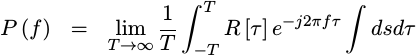 |
The good news is that this function can now easily be integrated across the new value s. The bad news is that the limits have become harder to calculate. For the sake of discussion, I’ll skip this bit of math and just point out that
 |
as long as  is less than
 T.
Now, since this PSD expression no longer depends upon T, we can take our limit and discover
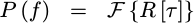 |
This is the conclusion of the Wiener-Khinchin theorem theorem.
What does this mean for the digital designer? Simple.
It means that if we estimate
,
we can later take a Fourier
transform of our estimate
in order to see what our
PSD
looks like.
But how to estimate
?
Estimating the AutoCorrelation Function
How shall we go about estimating
?
Let’s go back to the definition of
?
and first derive some properties of the
autocorrelation
function, then it should be easier to see how we might use this,
|
First, since we picked a function that wasn’t dependent upon time, we could just as easily write,
|
The first important property, and one that I’ve mentioned above, is that
.
I’ll leave this
proof for the student. The cool part about this property from a digital
designers standpoint is that we only need to estimate one half of
.
The other half we get for free.
Second, remember how we stated that an
expected value
could be approximated by an average? Suppose we kept track of some number of
prior samples of our signal, defined by however many values of
 we were interested in, and just averaged this product across
 N sample
pairs? We might then have
 |
If we skip the divide until later, we could rewrite this as,
 |
which looks very much like a value an FPGA might be able to calculate.
Here’s how this algorithm will work:
-
As samples come in, we’ll store them into an internal buffer–much like we did for the slow filter implementation.
-
Also, for each sample that comes in, we’ll read back an older sample, multiply the two together, and then add the result to a correlation accumulator held in memory indexed by the lag index,
.Note that the first time through, when the number of averages so far is zero, we’d need to write the product to memory rather than adding it to the prior value.
There is another, similar, implementation which we could build that would use a recursive averager here in order to have a result which is always available.
 |
Let me invite you to consider building this alternative implementation on your own and then comparing the results. Today, though, we’ll just build a straight block averager.
-
We’ll repeat this for some number of incoming averages,
N, that we want to calculate. -
Once we’ve reached the last average, we’ll stop, interrupt the CPU, and wait to be told to start again.
-
The CPU, can then read out the results and restart the spectral estimator to get a new estimate.
Optionally, we might choose to use a double-buffered design, similar to the one we used for the histogram in order to be able to always read out valid results, even when the algorithm is doing its calculations.
That’s the basics of the algorithm. Now, let’s see what it takes to schedule this pipeline.
Scheduling the Pipeline
As with a lot of algorithms of this type, such as any of our
slower filters,
we’re going to drive this from a state machine. The state machine will handle
when to start, how many averages need to be made, and so forth. The state
machine signals will then be used to drive a
pipeline
of operations for this
core.
Let’s allow that our state machine creates a signal, running,
which will be true as long as we continue our averages.
Now let’s work through the signals we might need. We can start with our product. This product will need both our new data, together with the data received by our design some number of clocks ago.
	always @(posedge i_clk)
		product <= delayed_data * new_data;
From just this operation alone, we can start working through an initial pipeline schedule.
 |
For example, once this operation is complete, we’ll then have a product that we need to add to the prior sum.
	always @(posedge i_clk)
		new_average <= last_average + product;
The product from our multiply will be available to create this new average on the clock after the multiply, and the new average will be available to be written to memory one clock after that. These values are shown in our initial schedule above, shown in Fig. 3.
A quick look at these signals will quickly reveal that they aren’t nearly
sufficient for an algorithm like this one. For example, where does the
delayed_data signal come from? It must be read from memory. That will
require a delayed signal address to be valid one clock earlier. Likewise, the
new data will need to be captured one clock earlier–but only at the beginning
of our run.
Let’s flesh this schedule out a bit more in Fig. 4 below.
 |
Moving one clock forward, in order to have a previous average in the “Product
Result” clock, we need an address in the prior clock period. I also chose
that prior clock period, “Product Operands”, to be the period where the
state variables would be valid, and so I created a running state flag
to indicate being in the state where I was walking through all of the
different lags, calculating a product on each lag.
Now, I can finally read the prior average,
	always @(posedge i_clk)
		last_average <= avmem[av_read_addr];
I also need to delay this address by two clocks within the pipeline in order to write the updated average data back, so I created a temporary address value to do this followed by the actual write address for the updated average data.
	initial { av_write_addr, av_tmp_addr } = 0;
	always @(posedge i_clk)
		{ av_write_addr, av_tmp_addr } <= { av_tmp_addr, av_read_addr};
That’s almost the whole
pipeline,
save one problem: on our first set of
averages, we want to make certain that we overwrite the average data.
This requires a flag, I’ll call it first_round, indicating that the
average data should be just the product of the data with the delayed data–not
that plus the prior average.
	always @(posedge i_clk)
	if (first_round)
		new_average <= product;
	else
		new_average <= last_average + product;
This first_round flag, however, has to come from our state machine which
… is valid one round prior. So, one round, prior I created a clear_memory
flag which would be true any time the number of prior averages, avcounts,
was zero.
At least, that’s the basic algorithm design.
Bootstrapping the Simulation
Formally verifying a DSP algorithm can be a real challenge simply for the fundamental reason that most formal verification tools can’t handle multiplies. Still, all I wanted from my design initially was to see a trace that would walk through all the operations of the core and set the interrupt output to indicate it had done everything. Consider how much work that takes to do in simulation,
//
// Definitions for reset_core, clear_mem, and request_start are
// defined above.
//
int	main(int argc, char **argv) {
	Verilated::commandArgs(argc, argv);
	TESTB<Vcheapspectral>	tb;

	//
	// ...
	//

	// Open a .VCD trace file, cheapspectral.vcd
	tb.opentrace(BASEFILE ".vcd");

	reset_core(&tb);

	int	iw, lglags, lgnavg, dmask, lags, navg;

	iw     = tb.m_core->o_width;
	lglags = tb.m_core->o_lglags; lags = (1<<lglags);
	lgnavg = tb.m_core->o_lgnavg; navg = (1<<lgnavg);
	dmask  = (1<<iw)-1;

	////////////////////////////////////////////////////////////////////////
	//
	// Test #1: Uniform (not Gaussian) noise
	//
	// Expected result: A peak at ADDR[&], much lower values everywhere else
	//

	clear_mem(&tb, lglags);
	request_start(&tb);

	// Set us up with completely random data, see what happens
	printf("Random data test\n");
	tb.m_core->i_data_ce = 1;
	for(int k=0; k<(lags+1) * (navg); k++) {
		tb.m_core->i_data    = rand() & dmask;
		tb.tick();

		if ((k & 0x3ffff) == 0)
			printf("  k = %7d\n", k);
	}
	tb.m_core->i_data_ce = 0;
	while(!tb.m_core->o_int)
		tb.tick();
Yes, I did eventually verify this core using simulation so I have the Verilator C++ code necessary to do it. But let’s now compare that to the amount of code necessary to just create a trace showing this design in operation using SymbiYosys,
	always @(*)
		cover(o_int);
Of course, when a cover() statement doesn’t produce the result you want,
you might find yourself in a bind not knowing what went wrong. So I added
a couple extra cover statements to help me know how long I would need to
wait for the outgoing
interrupt,
o_int, to be true.
	always @(posedge i_clk)
	if (f_past_valid && !$past(i_reset))
		cover($fell(running));

	// Let's verify that a whole round does as we might expect
	always @(*)
		cover(&avcounts);
There was one other key component to creating a trace of the logic within this
core
using SymbiYosys,
and that was reducing the number of lags checked and the number of averages
until the entire operation would fit into a reasonably sized trace.
While every tool has their own way of adjusting parameters at build time,
SymbiYosys
allows embedded Python scripts to accomplish the task.
Hence, the following lines in my
SymbiYosys
script
trimmed this cover() check down to something usable,
[script]
read -formal cheapspectral.v
read -formal fwb_slave.v
--pycode-begin--
cmd = "hierarchy -top cheapspectral"
if ("cvr" in tags):
	cmd += " -chparam LGLAGS 2"
if ("cvr" in tags):
	cmd += " -chparam LGNAVG 3"
output(cmd)
--pycode-end--
prep -top cheapspectral
The entire SymbiYosys script is posted, together with the algorithm on-line, so feel free to examine it and compare with the Verilator simulation code.
As I mentioned above, I also ran simulations on this core (eventually), but we can come back to that in a moment. For now, let’s back up and discuss the state machine signals for a moment based upon the trace SymbiYosys generated and shown below in Fig. 5.
 |
The whole operation starts out with a start_request, set by either the bus
or a reset. This start request clears the count of the number of averages,
avcount, sets a flag to indicate that we’ll be clearing our average memory,
clear_memory, and sets another flag to indicate that we wish to be responsive
to the next data item that comes in, check_this.
Once a new data value comes in, as indicated by
i_data_ce && !running && check_this, the
core
starts calculating products and adding them to the running
autocorrelation
accumulators. Once it has gone
through all of the various lags contained in those accumulators,
the core
then waits for another data item to come in.
What if other data items come in while
the core
is busy? They are ignored.
We can do this because we’ve already assumed that our signal was
wide-sense stationary,
and so which value we use to run our estimates on
shouldn’t matter, right? Well, there is an unfortunate consequence to this.
Specifically, if you provide
the core
with a cyclostationary
signal,
one whose statistics repeat in time every 1+2^LGLAGS system clocks, you might
not get a representative result. If you think that’s your case, you can
include a random number into the start check, so as to randomly spread out
which values you check and thus guarantee a more uniform rather than periodic
sample set–but that would be a (slightly) more advanced design than the
one we are working on today.
Suppose we zoom in on this trace a bit more, and see what’s going on while
the core
is running? There’s a lot that happens there, and it’s worth
understanding.
 |
First, any time new data comes in, it is written to memory and the
data_write_address is incremented. If that new data comes in when the
autocorrelation
updater is already running, it simply gets written
to memory but otherwise ignored. This is why the new_data trace above
can appear to skip values, such as jumping from D4 to D9, but also
increment from one value to the next, such as from D9 to DA to DB
when the data arrives slow enough.
If the averager isn’t running, however, this new data sample is taken to run
correlations on with past data. It’s important, for
pipeline
purposes, that
the delayed_address be one greater than the data_write_address on this
clock. That helps to guarantee that no matter what data comes in while we
are processing, the most recent data will always be read back in time to
calculate a zero lag. You can see this in Fig. 6 above by the fact that the
delayed_data that’s read from memory always equals the new data on the last
period while the design is running–regardless of how fast new data comes in.
On the clock period after the running state machine signal, the address
of the prior average for this lag is valid. That gets read into last_average
on the next clock, and then added to the product and written out on the
clock after as the new_average.
That’s essentially all of the major design details. The cool part is that
I was able to see all of these details from the cover() trace produced
above–at least enough to organize it into the charts you see in both
Figs. 5 and 6 above.
Let’s walk through how all this logic fits together into the next section.
The Cheap Spectral Estimator Design
If you aren’t interested in the gory details of this algorithm, feel free to skip forward a section to see how well the algorithm works. On the other hand, if you want to try building something similar, you might enjoy seeing how the inner details work. Surprisingly, they aren’t all that different from how our prior slow filter worked: there’s one multiply that’s shared across operations and some block RAMs to contain any data we need to keep track of.
Our core’s portlist footprint isn’t really much more than that of any generic
Wishbone slave. The
biggest difference is that we have the i_data_ce signal
to indicate new data is valid, and the i_data signal containing any new
samples from our signal.
module	cheapspectral(i_clk, i_reset,
		i_data_ce, i_data,
		i_wb_cyc, i_wb_stb, i_wb_we, i_wb_addr, i_wb_data, i_wb_sel,
			o_wb_stall, o_wb_ack, o_wb_data,
		o_int);
We also output an
interrupt,
o_int, any time
the core
completes its averaging and has an
autocorrelation
estimate available to be examined.
Next, we’ll need to decide how we want to configure this core.
First, we’ll need to know how many lags we wish to check. That is, how big, or rather how long, should our correlation function estimate be? This is important. The more samples in your estimate, the more freuency “resolution” your PSD will have, but also the longer it will take the result will take to converge.
The parameter of LGLAGS=6 sets the number of lags calculated to 2^6 = 64.
It’s not amazing, but it will work for most testing and verification purposes.
parameter LGLAGS = 6;We’ll also allow our incoming data to have an implementation dependent bit-width.
parameter IW = 10; // Input data WidthFinally, we need to know how many averages to do. The more averages you do, the less jumpy the resulting estimate will be and the closer it will hold to the actual autocorrelation. However, the more averages you do, the longer it will take to get an estimate of your signal. You, as the designer, will need to make that tradeoff.
Here, we just specify the number of averages as a log based two number.
Fifteen this corresponds to averaging 2^15 = 32,768 points together to
get our spectral estimate.
parameter LGNAVG = 15;Again, this only works if the incoming signal truly was wide-sense stationary. While very few signals truly are, the approximation is still useful in real life. Just beware that if the environment changes mid-average, then you won’t necessarily see the change in the results.
Two more parameters, the number of address bits for our bus interface and the width of the bus, are just useful for making the design easier to read below.
	localparam	AW = LGLAGS;
	localparam	DW = 32;	// Bus data width
For your sake, I’ll spare the port and signal definitions that follow, but you are more than welcome to examine the details of the core itself if you would like.
The first block of logic within the core involves writing incoming data to memory. Every new data value will get written to memory regardless of whether or not it drives a summation round below.
	initial	data_write_address = 0;
	always @(posedge i_clk)
	if (i_data_ce)
		data_write_address <= data_write_address + 1;

	always @(posedge i_clk)
	if (i_data_ce)
		data_mem[data_write_address] <= i_data;
Note that there’s no reference to the reset signal here. This was a careful design choice made on purpose. First, you can’t reset block RAM. Sorry, it just doesn’t work. Second, any data flow will (eventually) work its way through whatever junk was in the data registers initially. Finally, this logic keeps our last read data values always valid.
Where it gets annoying is when we try to build a simulation with a known input and a (hopefully) known output, but that’s another story.
The next piece is the start request that starts off our whole estimate. This core will immediately estimate the autocorrelation of an incoming waveform immediately on startup, on reset, or upon any write to the core.
		initial	start_request = 1;
		always @(posedge i_clk)
		if (i_reset)
			start_request <= 1'b1;
		else if (i_wb_stb && i_wb_we)
			start_request <= 1'b1;
Once the core has started running in response to this start request, the request line will clear itself.
		else if (!running && i_data_ce && check_this)
			start_request <= 1'b0;
The check_this signal below is used to indicate we want to calculate an
autocorrelation
estimate. It gets set on any start request, but also
automatically clears itself after the last average. In this fashion,
we can hold onto an average until it is read before using it again.
	initial	check_this = 1;
	always @(posedge i_clk)
	if (i_reset)
		check_this <= 1'b1;
	else if (!running)
		check_this <= (check_this || start_request || !(&avcounts));
	else
		check_this <= !(&avcounts);
Once we’re all done, we’ll want to set an
interrupt
wire for the
CPU to
examine. That’s the purpose of o_int below. It will be set during the
last average set once the last value is written to the average memory.
	initial	o_int = 0;
	always @(posedge i_clk)
	if (i_reset || start_request)
		o_int <= 1'b0;
	else
		o_int <= update_memory && last_write && (&av_write_addr);
The next item in our state machine is the counter of the number of averages we’ve calculated. We’ll clear this on any start request, and otherwise increment it at the end of any processing group–as shown in Fig. 5 above.
	initial	avcounts = 0;
	always @(posedge i_clk)
	if (i_reset)
		avcounts <= 0;
	else if (!running)
	begin
		if (start_request)
			avcounts <= 0;
		else if (i_data_ce && check_this)
			avcounts <= avcounts + 1;
	end
As shown in our
pipeline
schedules and figures above, its important to calculate
the address for the prior signal data, delayed_addr, so that it’s valid
when !running. Further, it needs to be valid on all but the last clock of
running. Finally, the value is critical. When the data that we are going
to examine gets written, that is when i_data_ce && !running, this address
must already be equal to the next data memory address following the write
address. That helps to 1) give us immunity to the data speed, while also
2) guaranteeing that the last value we examine is the value just received and so
contributes to the R[0] average.
The extra variable here, last_read_address, is used as an indication
that we need to base the next value on the current address of the next
data that will come in, data_write_address, rather than just continuing
to walk through older data.
	always @(posedge i_clk)
	if (running && !last_read_address)
		delayed_addr <= delayed_addr + 1;
	else
		delayed_addr <= data_write_address + 1
			+ ((i_data_ce && check_this) ? 1:0);

	always @(*)
		last_read_address = (running && (&av_read_addr[LGLAGS-1:0]));
The address for the reading from the average accumulator memory is called
av_read_addr. We always walk through this address on every run from start,
av_read_addr==0, to stop, &av_read_addr. When not running, we go back
to the first address to prepare for the next round.
		always @(posedge i_clk)
		if (running)
			av_read_addr <= av_read_addr + 1;
		else
			av_read_addr <= 0;
If you look through the trace in Fig. 6 above, there’s really an extra clock in there over and above what needs to be there. This is one of those pieces of logic that would need to be updated to get rid of that extra clock.
Personally, I’m okay with the extra clock if for no other reason than the
number of clock cycles required for any averaging cycle, 1+2^LGLAGS, tends
to be relatively prime to most digital artifacts and so (perhaps) keeping
it this size will help reduce any
non-WSS
artifacts.
That really only leaves two state machine signals left to define, the
running and clear_memory flags. As you may recall from our
pipeline
schedule, running will be true while we are working through the various
products of our
autocorrelation
estimate. It gets set whenever new data
comes in that we are expecting, i.e. whenever i_data_ce && check_this value.
It gets cleared once we read from the last address of our
autocorrelation
average memory.
The clear_memory flag has a very similar set of logic. This is the flag
that’s used to determine if we want to rewrite our accumulators versus
just adding more values to them. For the first averaging pass, we’ll want
this value to be set–so we set it on any reset or following any
start_request. We then clear it at the same time we clear the running
flag.
	initial	running = 1'b0;
	initial	clear_memory = 1'b1;
	always @(posedge i_clk)
	if (i_reset)
	begin
		running <= 1'b0;
		clear_memory <= 1'b1;
	end else if (running)
	begin
		if (last_read_address)
		begin
			running <= 0;
			// If we were clearing memory, it's now cleared
			// and doesn't need any more clearing
			clear_memory <= 1'b0;
		end
	end else // if (i_data_ce)
	begin
		running <= i_data_ce && check_this;
		if (start_request)
			clear_memory <= 1'b1;
	end
Finally, in order to know when to write to our memory, we’ll want to delay
the running indicator through our
pipeline.
That’s the purpose of the run_pipe signal below.
	initial	run_pipe = 0;
	always @(posedge i_clk)
	if (i_reset)
		run_pipe <= 0;
	else
		run_pipe <= { run_pipe[0], running };
It’s now time to walk through the various stages of the pipeline processing.
If you examine the code, you’ll see I’ve placed a comment block at the beginning of the logic for each pipeline stage, to help me keep track of what’s being done when. Indeed, this was how I originally scheduled the pipeline in the first place–I only drew Fig. 3 after the entire design was up and running.
	////////////////////////////////////////////////////////////////////////
	//
	//
	// Clock 0 -- !running
	//	This is the same clock as the data logic taking place above
	// Valid this cycle:
	//	delayed_addr, i_data_ce, i_data
	//
After getting the various signals associated with each clock wrong a couple
of times, I started adding to the comment block the list of signals defined
by each block. When that wasn’t enough, I then added to the block the signal(s)
that defined when the
pipeline
stage was active. In this case, clock 0
takes place one clock before the running clock, as shown in Fig. 4 above
in the cycle I called “Incoming data”.
It’s on this clock that we need to copy the incoming data to our new_data
register, to be used in our subsequent
autocorrelation
calculations. This
helps to make certain that it doesn’t change on us while running.
	always @(posedge i_clk)
	if (!running)
		new_data <= i_data;
Similarly, we’ll want to read the delayed data from memory.
	always @(posedge i_clk)
		delayed_data <= data_mem[delayed_addr];
It’s on the next clock that we’ll multiply these two values together.
	////////////////////////////////////////////////////////////////////////
	//
	//
	// Clock 1 -- running
	// Valid this cycle:
	//	new_data, delayed_data, clear_memory, av_read_addr
	//
The biggest and most important part of this next clock cycle is multiplying our two data values together.
`ifdef	FORMAL
	(* anyseq *) wire signed [2*IW-1:0]	formal_product;

	always @(posedge i_clk)
		product <= formal_product;
`else
	always @(posedge i_clk)
		product <= delayed_data * new_data;
`endif
Notice how I have two versions of this multiply above. The first version, used when we are using formal verification, allows the multiplication result to be (roughly) anything. (I constrain it more in the formal section that follows.) The second version is how it would work normally.
The clear_memory flag is true on this clock, but we won’t add this product
together with the lag product for another clock. On that clock we need to know
if it’s the first round or not, so let’s move this value one clock further
into our
pipeline.
	initial	first_round = 1'b1;
	always @(posedge i_clk)
		first_round <= clear_memory;
The last thing we need from this clock cycle is the previous value from the accumulator memory. That’s as easy as just reading it.
	initial	last_average = 0;
	always @(posedge i_clk)
		last_average <= avmem[av_read_addr];
Unlike the histogram design, we don’t need to worry about operand forwarding during this calculation. When we read this value, we can rest assured that it won’t also be present in any of the two subsequent stages. That will nicely simplify the logic that follows.
	////////////////////////////////////////////////////////////////////////
	//
	//
	// Clock 2 -- $past(running), run_pipe[0], product is now valid
	// Valid this cycle:
	//	product, first_round, last_average, av_tmp_addr, last_tmp
	//
Moving on to the next clock, we now want to add our product and last average together.
	assign	calculate_average = run_pipe[0];

	always @(posedge i_clk)
	if (first_round)
		new_average <= { {(LGNAVG){product[2*IW-1]}}, product };
	else
		new_average <= last_average
			+ { {(LGNAVG){product[2*IW-1]}}, product };
I’ve chosen to be explicit with the sign bit extensions here to avoid
Verilator
warnings, but this should be equivalent to last_average + product.
I also need to move the accumulator read address from the last
pipeline
stage into the next one. This can be done with a simple shift register,
although I’ll admit I did get the length of this register wrong once or
twice. This is now the correct width with av_tmp_addr having the same
number of bits as av_write_addr.
	initial { av_write_addr, av_tmp_addr } = 0;
	always @(posedge i_clk)
		{ av_write_addr, av_tmp_addr } <= { av_tmp_addr, av_read_addr};
The last task in this
pipeline
stage is to determine if this is the last write block. If it is, we can set the
interrupt
above. It would be a bit of a problem, however, for the
CPU to restart this
core
only to get an interrupt
from a prior calculation. To suppress this extra
interrupt, we reset this
flag on either a system reset, i_reset, or a user restart of the
core.
	initial { last_write, last_tmp } = 0;
	always @(posedge i_clk)
	if (i_reset || (i_wb_we && i_wb_stb))
		{ last_write, last_tmp } <= 0;
	else
		{ last_write, last_tmp } <= { last_tmp, (&avcounts) };
That brings us to the third clock.
	////////////////////////////////////////////////////////////////////////
	//
	//
	// Clock 3 -- run_pipe[1], new_average is now valid
	// Valid this cycle:
	//	new_average, update_memory, av_write_addr, last_write
	//
During this clock, all we need to do is write the data back to memory.
	assign	update_memory = run_pipe[1];

	always @(posedge i_clk)
	if (update_memory)
		avmem[av_write_addr] <= new_average;
When should we write? Two clocks after running–which is what run_pipe
keeps track of for us.
The last piece of this core is handling bus interactions.
	////////////////////////////////////////////////////////////////////////
	//
	// Handling the bus interaction
	//
	////////////////////////////////////////////////////////////////////////
	//
	//
If you are using Wishbone, this is really easy. Indeed, it’s as easy as the simple Wishbone slave we discussed some time ago.
We hold the stall line low,
assign o_wb_stall = 1'b0;and acknowledge any bus request one clock later.
	initial	o_wb_ack = 1'b0;
	always @(posedge i_clk)
		o_wb_ack <= !i_reset && i_wb_stb;
I know the original simple Wishbone
slave
didn’t have the check on i_reset,
but I’ve learned a bit since using
formal methods.
Two particular things
formal methods
have taught me are first to use the initial value, and second
to reset the acknowledgment.
The last step would be to read data from the averages register. Ideally, this should look like,
	always @(posedge i_clk)
		o_wb_data <= avmem[i_wb_addr];
Except … that’s not good enough. In particular, the average memory, avmem,
has a width given by 2*IW+LGNAVG which might or might not match the bus
width of `o_wb_data.
So I’m going to read into a register of exactly the right length first,
		always @(posedge i_clk)
			data_out <= avmem[i_wb_addr];
and I’ll expand into the right width in the next step.
If the two widths match, I can just keep o_wb_data the same as this
data_out value.
	generate if (AB == DW)
	begin : PERFECT_BITWIDTH

		always @(*)
			o_wb_data = data_out;
At the next step, though, I need to admit I broke a working design by not doing this right. Obviously, if there aren’t enough bits, you’d want to sign extend to the right number of bits.
	end else if (AB < DW)
	begin : NOT_ENOUGH_BITS

		always @(*)
			o_wb_data = { {(DW-AB){data_out[AB-1]}}, data_out };
Here’s the problem I ran into: I was running simulation tests with
2^1024 lags and 10 bit data, and 1024 averages. When simulations took
too long and the data didn’t quite look right (it was close), I adjusted
the design to examine 2^64 lags and 32768 averages. All of a sudden
my correlation results were all broken.
As an example, if you give the core a sine wave input, you should be able to read a cosine autocorrelation output, as shown in Fig. 7.
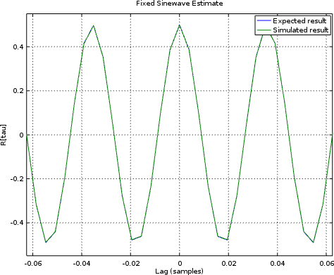 |
However, when I looked at the autocorrelation of a sinewave, I received the autocorrelation output shown in Fig. 8 below.
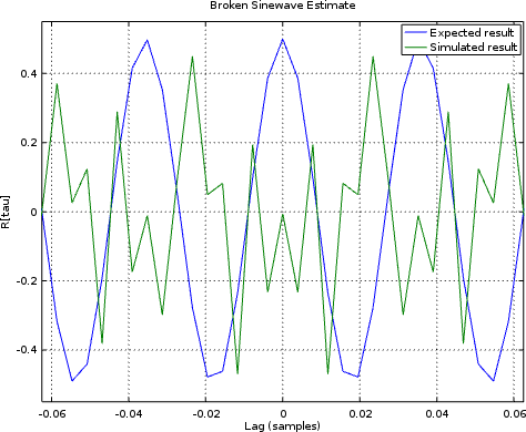 |
The first indication that something is broken is the fact that R[0]
isn’t a maximum. The second indication, the fact that the measured waveform
looks nothing like what it should.
It took me quite a bit of time to find this bug. It got so far that I was
chasing it in a simulation waveform, and the
autocorrelations all looked
right. Then I noticed the number of bits in data_out–35. The top three
bits were getting dropped in the assignment above (which wasn’t originally
contingent on the number of bits).
A sadder man but wiser now, I’ve learned to check for all possible differences
between the number of bits in data_out and the bus width. The check above,
and the third case (below) fixes this issue.
	end else begin : TOO_MANY_BITS

		always @(*)
			o_wb_data = data_out[AB-1:AB-DW];

		wire	unused;
		assign	unused = &{ data_out[AB-DW-1:0] };
	end endgenerate
That’s the logic necessary to build this core.
endmoduleBut does it work?
Simulation Results
If you look over the
core,
you’ll find a formal proof that the R[0] value is positive, and that
the accumulator hasn’t overflowed. While that’s nice, it doesn’t really
compare the
core’s
performance against a known input to know that it produces a known
output. To handle that, I tried seven known inputs using a
Verilator simulation script.
-
Random Noise
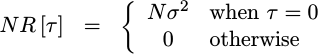
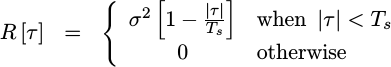
The classic autocorrelations test is random noise. If noise values have a known variance,
 |
and if noise values are equally likely positive as they are negative, then it’s not all that hard to prove that the correct correlation would be given by,
 |
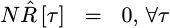
Of course, this is only the true autocorrelation, depending upon the mathematical expectation operator, which itself is dependent upon a fictitious probability density function which may or may not match reality. Unfortunately, the algorithm above only estimates the autocorrelation and the estimate may or may not equal the expected value. Sure, over time it will get closer, but how shall I easily tell if the current value is close enough to declare that my simulated algorithm “passes” its simulation check?
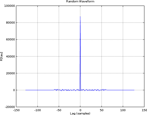 |
Having the right shape above is at least a good start, so let’s keep going.
-
All zeros
After my frustrations with the random data, I thought to try some carefully chosen known inputs for testing. The easiest of these to work with was the all zeros incoming sequence. Clearly if the inputs are all zero, then the autocorrelations estimate should be zero as well.
 |
Unfortunately, the all zeros sequence doesn’t really create anything pretty to plot and display. Hence, while the test (now) works, it doesn’t leave much to show for it.
-
All ones
The problem with the all zeros sequence is just the large number of broken algorithms that would still pass such a test. Therefore I thought I’d create a third test where the inputs were all ones. As with the all zeros test, the result should be absolutely known when done.
 |
Sadly, as with the all zeros test, the result isn’t very interesting and so not really worth plotting.
-
Alternating ones and negative ones
What if we alternate plus and minus ones on the input? Again, the estimate of the autocorrelations should match the actual autocorrelations, with
 |
Now we can finally plot something of marginal interest. In this case, we can also compare the expected autocorrelation against the measured one.
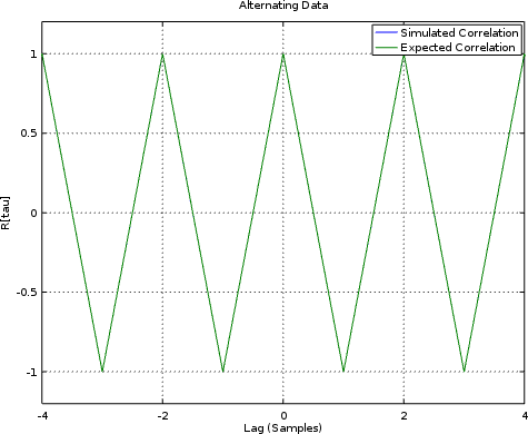 |
The two are clearly shown on top of each other, so we can mark this test down as a success.
-
Alternating ones and negative ones, only slower
I then tried to create a similar signal that would alternate ones and negative ones, just slower: seven
1s followed by seven-1s in a repeating sequence. The only problem was, I didn’t really work out the math to know what the “right” answer was or should be. As a result, although I can plot the result, it’s harder to tell whether it works or not. -
A Sinewave
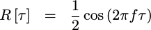
That leads to another autocorrelation test that might be of interest: what would happen if we gave this algorithm a sinewave as an input?
 |
This is another one of those “classic” inputs, where the result should match a known pattern. Indeed, with just a little math, it’s not hard to prove what the autocorrelation result should be.
 |
Unfortunately, as with the first test case, the core will only produce an estimate of the true autocorrelation function, rather than an exact autocorrelation result. Worse, with a little work, you’ll realize that multiplying two sine function values together will result in a cosine plus another trigonometric term. The second term should average out, but I haven’t yet tracked out what it’s limits are and whether or not the average is causing this second term to average out as fast as it should.
Still, if you compare the sinewave spectra with the expected spectra in Fig. 11 below, the two land nicely on top of each other.
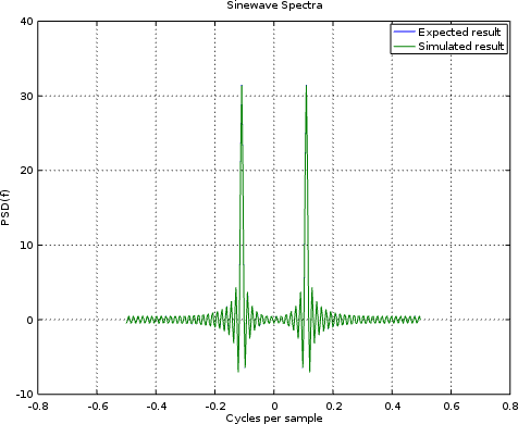 |
That suggests that we’re at least on the right track.
I will admit that when I looked at this shape for the first time I was a little confused. The “correct” spectra for a sinewave should be a single peak, right?
Sadly, no. The “correct” spectra of a sinewave should be two peaks–one at the positive sinewave frequency and one at the negative frequency. (I was using complex FFTs.) Not only that, but the sinewave’s spectra should consist of two sinc functions superimposed upon each other, and so this result does look right–even if it wasn’t what I was expecting at first.
-
A Random Binary Waveform
Let’s finally move on to a last test case, and pick something more likely to be a useful demonstration. So, let’s pick a random binary waveform. This waveform will contain a series of bit-periods where the input to the core will be either plus or minus full scale,
+/- (2^{IW-1}-1).As with the sine wave, the true autocorrelation of such a waveform has a closed form representation,
 |
where sigma^2 is the absolute value of the signal.
Much to my chagrin, I only got close to this estimate, as shown in Fig. 12.
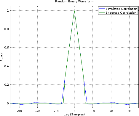 |
Was it close enough? Perhaps, but what I’d really like to do is to display the PSD of such a signal, as shown in Fig. 13 below.
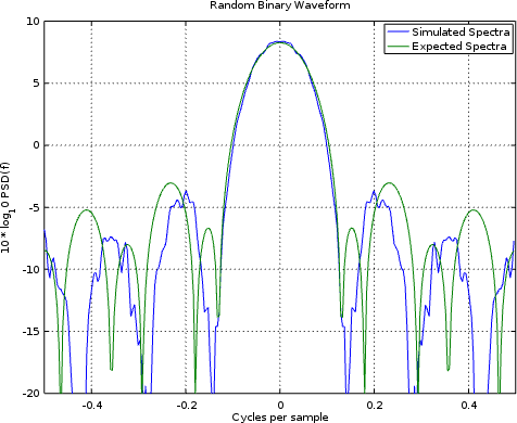 |
In this case, we got close again. Unfortunately, it wasn’t close enough to match the expected shape over 10dB down.
Still, all told, we’ve done a decent job of estimating the PSD of a signal within our FPGA, but without actually running any FFTs on the FPGA to do it.
Conclusion
If your goal is to grab a picture of what the spectral content is of a signal within your design, but without using a lot of logic, then I’d say we’ve achieved it with this little design. No, it’s not perfect, and yes there’s some amount of variability in the estimated waveforms–this is all to be expected. The cool part is that this technique only uses one multiply and a couple of block RAM memories.
Will this fit on an iCE40 UP5k, together with other things? Indeed, there’s a good chance I’ll be able to add this in to some of my SDR designs to “see” what’s coming in from the antenna. Indeed, given the speed and simplicity of this algorithm, I might even be able to handle the incoming data at the 36MHz data rate! There’s no way I could’ve done that with an FFT approach–not on this hardware at least.
Only they would that we should remember the poor; the same which I also was forward to do. (Gal 2:10)