
A CORDIC testbench
Some time ago, I presented a CORDIC algorithm on this blog. This CORDIC algorithm makes it possible to generate sine and cosines using normalized integers as phase angles and only additions and shifts. The CORDIC algorithm is unique because of the simple fact that it does not require any multiplies to calculate these trigonometric values.
Since that time, we’ve demonstrated the utility of this algorithm when testing a proposed/modified PWM algorithm.
This is only the beginnings of what a CORDIC algorithm can be used for. You can also modulate baseband signals to intermediate/carrier frequencies, and downconvert them back to base band, using the same approach. It is really quite versatile.
CORDICs can also be used for generating test functions for FPGA based filters. This is particularly where I’d like to go with the technology on this blog. This means that our filtering test bench will depend upon this CORDIC algorithm, and hence any failure in the CORDIC will have a ripple affect into our future articles.
For this reason, we need to get the CORDIC test bench right.
It also turns out that we made our problem more difficult by creating a core generator approach to our CORDIC algorithm. Because of the core generation approach, our CORDIC test bench will need to run across all manner of parameters: number of stages, input data width, phase bit-width, extra internal bits, and output bit width. So that we could handle this extra variability, we took a pause in our development in order to present some probabilistic quantities related to quantization which we can now use to predict the performance we expect so as to measure how well we do in comparison to it.
Building this test bench is going to take several steps. The first several of those will estimate how close we can expect the CORDIC algorithm to get to the right result. This is important, because it will then form the basis for any performance thresholds we might create to know if our implementation works. These results can also be used as an estimate of how well the CORDIC algorithm will perform for arbitrary input parameters.
Hence, after discussing both what quantization and phase variance one might expect, we’ll turn our attention to building the actual test bench.
Theorem Rules
A previous post put together a couple of probabilistic formulas and variance rules. Let’s just reiterate these for background here.
-
Quantization noise has a variance given by
1/12th of a perfect Analog to Digital Converter (ADC)’s step size. -
The variance of a random variable multiplied by a constant is given by the variance of that variable times the constant squared.
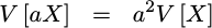
This applies to all random variables.
-
We’ll assume that any random variables we deal with are independent.
-
The variance of the sum of two random variables is given by the sum of the variances:

This follows from our assumption that the two random variables,
XandY, are independent. -
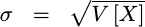
The standard deviation of a random variable is given by the square root of the variance.
These will form the basis of the error estimation work that follows. Indeed, we’ll use several of these properties at every step.
From Core Generator to Test Bench
One of the hassles of any test bench for a core generated algorithm is communicating information from the core generator to other parts of the design, such as the test bench. The problem has a simple solution.
The approach we’ll take for dealing with this problem is to have the
core generator generate
not only the CORDIC
code itself, but also a
C header file
describing the relevant choices that were made in the
core generator.
The core generator
will create this C header
file
any time the command line parameter -c is given to it.
The basic information found within this
file
includes the bit widths of the input (IW), output (OW), and phase (PW).
It also includes the number of extra bits, NEXTRA,
used in the CORDIC
computations, as well as the number of
CORDIC
stages, NSTAGES. Finally, this
header file
will contain information regarding whether or not the reset wire
or the traveling
CE
wire (aux) were included within the design.
We’ll add to this basic information some probabilistic prediction information we’ll develop below.
You can see an example of such a C header file, produced by our core generator, here.
Input Quantization
Now let’s start our run through the various errors or noise sources within the CORDIC algorithm.
The first noise source is the
quantization
of the input samples. We can assume that both i_xval and i_yval come with
an input quantization
variance
of 1/12th–as we discussed in our last
post. Likewise, the
variance of the phase is 1/12th of
the lowest phase unit squared.
In our
CORDIC algorithm,
though, our first step was to multiply these input values by a programmable
number of extra bits. The number of these extra bits was used to create a
working width, WW, used below,
// WW is the number of XTRA bits plus the maximum of IW and OW
// These lines therefore add XTRA bits to our values
//
wire signed [(WW-1):0] e_xval, e_yval;
assign e_xval = { {i_xval[(IW-1)]}, i_xval, {(WW-IW-1){1'b0}} };
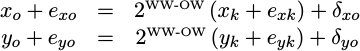
assign e_yval = { {i_yval[(IW-1)]}, i_yval, {(WW-IW-1){1'b0}} };To express this mathematically, we’ll let x_i and y_i represent the
inputs to the algorithm, and x_0 and y_0 represent the inputs to the first
rotation. Since the precision of these values is not affected by the
pre-rotation step, no additional error is inserted there. Hence, we have the
following representation for the inputs to our first rotation:
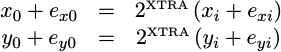 |
In this equation, e_xi and e_yi are any errors associated with the
inputs x_i and y_i. Once the multiply has been accomplished, we’ll
express the output as a sum of both the desired output x_0 and y_0,
together with the differences from perfection, e_x0 and e_y0. These latter
two random values
are the errors in our precision following this step.
Using our variance
rule for multiplying an input by a constant, the
variance
of these two error terms, e_x0 and e_y0, is then given by,
 |
This is the then variance at the input to our CORDIC rotation stages.` From here we’ll move to the rotation steps themselves.
Internal Truncation Error
The next source of error within our CORDIC implementation may be found within the CORDIC rotation stages themselves.
As you may recall, each
CORDIC stage
rotates the previous x,y values using a transform matrix using the equations:
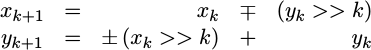 |
There was also a corollary transform for when we wished to rotate in the other direction. To represent both, we used the plus-or-minus character above. Further, the minus-or-plus character above captures the fact that two separate signs need to change together, but that they need to be opposites of each other.
However, while this was the rotation equation we presented, it wasn’t quite what our FPGA code accomplished within our implementation.
if (ph[i][(PW-1)]) // Negative phase
begin
	// If the phase is negative, rotate by the
	// CORDIC angle in a clockwise direction.
	xv[i+1] <= xv[i] + (yv[i]>>>(i+1));
	yv[i+1] <= yv[i] - (xv[i]>>>(i+1));
	ph[i+1] <= ph[i] + cordic_angle[i];
end else begin
	// On the other hand, if the phase is
	// positive ... rotate in the
	// counter-clockwise direction
	xv[i+1] <= xv[i] - (yv[i]>>>(i+1));
	yv[i+1] <= yv[i] + (xv[i]>>>(i+1));
	ph[i+1] <= ph[i] - cordic_angle[i];
end
Within our
implementation,
we truncated the values of x_k and
y_k after shifting them to the right. This is equivalent to adding
random variables,
d_xk and d_yk to each of the x_{k+1} and y_{k+1}
values in addition to the error terms brought to this stage from the prior
stage. We can separate the desired result, x_(k+1) and y_(k+1) from the
accumulated errors in the result, e_x(k+1) and e_y(k+1) and re-represent
this as,
 |
Using our addition of variances rule, together with the scale rule, we can calculate a variance for the error term at the end of this stage.
![V[e_x] = (1+2^(-2k))*v[e_k]+V[d_k]](/img/cordic/eqn-cordic-stage-variance.png) |
At this point, we know V[e_k] from the previous stage, and with the
exception of V[d_k] we can calculate V[e_(k+1)] for the next stage.
But … what is V[d_k]?
Unlike the
quantization
error we calculated earlier, truncation error is neither zero
mean
nor does it have a 1/12
variance.
However, if we assume that the choice of direction is made randomly,
with a probability of one half for each rotation direction, then the truncation
error becomes zero
mean.
(Half the time the
mean
is negative by one half, half the time it is positive by one half, etc.)
The variance,
though, is given by 1/3 since we need to integrate from
0 to 1 instead of from -1/2 to 1/2:
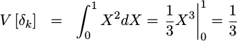 |
Well, okay, that’s close but not quite right. In reality, the truncation
error associated with truncating an already
quantizated
number requires an analysis of a discrete probability
distribution.
If we suppose that a finite number of bits, k, are dropped in the
truncation then the variance is not 1/3rd but
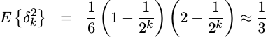 |
The proof of this doesn’t fit on a single line, however, so we’ll leave the details as an exercise for the student.
After the CORDIC rotation stages, we rounded the result and produced an ouput. That step, therefore, is next.
Output Variance
The last step in calculating the variance of the CORDIC’s output, is to adjust the resulting output variance due to the last rounding step:
assign	pre_xval = xv[NSTAGES] + { {(OW){1'b0}},
			xv[NSTAGES][(WW-OW)],
			{(WW-OW-1){!xv[NSTAGES][WW-OW]}}};
assign	pre_yval = yv[NSTAGES] + { {(OW){1'b0}},
			yv[NSTAGES][(WW-OW)],
			{(WW-OW-1){!yv[NSTAGES][WW-OW]}}};

always @(posedge i_clk)
begin
	o_xval <= pre_xval[(WW-1):(WW-OW)];
	o_yval <= pre_yval[(WW-1):(WW-OW)];
	o_aux <= ax[NSTAGES];
end
As you may recall, WW was the working width we were using for the
CORDIC
transform stages, and OW is the output width. If WW is greater than OW,
then this stage drops bits and rounds the result. This rounding step also
adds some more
quantization
variance.
Mathematically, we might write what is taking place with,
 |
At this point, we know the
variance
of just about all of the components.
x_k and y_k are fixed values (not random), so their
variance is zero.
The variance
e_xk and e_yk were both calculated in the last step.
Using our
scale and addition rules,
we can express the final
variance as,
 |
The variance
of d_xo is the only thing left to discuss. This is the
variance
associated with our rounding step. If we treat the value as continuous, then
the
variance
of d_xo would be 1/12th. This isn’t quite the case, since
d_xo is quantized, but it makes a decent approximation. (The actual number
starts at 1/8 for dropping one bit, and asymptotes at 1/12 for dropping
an infinite number of bits.)
We can now use this value to calculate the variance both at the end of each CORDIC stage, as well as at the end of the entire algorithm. We’ll place the code to calculate this value within our generic CORDIC library:
double	transform_quantization_variance(int nstages, int xtrabits, int dropped_bits) {
	double	current_variance;

	current_variance = pow(2,2*xtrabits)/12.;

	for(int k=0; k<nstages; k++)
		current_variance = (1+pow(4,-k-1))*current_variance + 1/3.;

	// If we drop bits from this on the output, then we add more variance
	// in the process.  This is rounding variance, so the variance is
	// (roughly) 1/12th.
	if (dropped_bits > 0)
		current_variance = pow(2,-2*dropped_bits)*current_variance + 1/12.;
	return current_variance;
}
The result of this calculation will be passed to the test
bench
by passing a QUANTIZATION_VARIANCE value to the test
bench
within our core-generated
header file:
const double QUANTIZATION_VARIANCE = <actual value goes here>; // (Units^2)This will then inform our test bench code the average sum of square errors that it can expect.
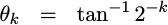
At this point, we’re almost done with our pre-work. We have only one step left, and that is looking into any variance associated with the phase accumulator.
Phase Error
There’s one last component to the
variance
of our result, and that’s the
variance
associated with the phase accumulator. You may recall that, at each
stage of our
CORDIC algorithm, we added
or subtracted an amount of phase to a phase accumulator. We calculated
these phase values within
cordiclib.cpp
and placed these values into the cordic_angle array within our generated
routine.
 |
The problem with this array is that the phase values had to be quantized in order to be placed into this integer array. This quantization can be found within our CORDIC library:
void	cordic_angles(FILE *fp, int nstages, int phase_bits) {
	// ...

	for(unsigned k=0; k<(unsigned)nstages; k++) {
		double		x;
		unsigned long	phase_value;

		x = atan2(1., pow(2,k+1));
		// ...
		// Convert this value from radians to our integer phase units
		x *= (4.0 * (1ul<<(phase_bits-2))) / (M_PI * 2.0);

		// Here's where we truncate our phase from a double to an
		// integer.
		phase_value = (unsigned)x;
		// ...
	}
	// ...
}
This means that though we intended to rotate by one angle,
we ended up rotating by an approximation of that angle. If we let
gamma reference the
CORDIC
gain, R(theta) represent the rotation we
wanted to accomplish, and e_ox and e_oy be the algorithm errors we’ve
been discussing so far, then our result should be:
![[X,Y] = gR(theta)+errs](/img/cordic/eqn-cordic-desired.png) |
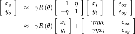
The problem with this representation is that it doesn’t acknowledge any of these phase errors. In other words, because we’ve only approximated the phase errors with integers, we ended up rotating by a different phase–one that was close to what we wanted to rotate by:
![[X,Y] = gR(theta+eta)+errs](/img/cordic/eqn-cordic-err-rotation.png) |
If we separate the rotation into two rotations, one by the rotation we want,
R(theta), and the other by the rotation we didn’t want, R(eta), we can
rewrite this as:
![[X,Y] = gR(theta)R(eta)+errs](/img/cordic/eqn-cordic-rotation-separated.png) |
Finally, if we use a small angle approximation for eta, then this can be
rewritten as something a touch more useful:
 |
At this point, our results are separated between the results we want, together
with an additive “noise” term that we didn’t want. From here, then, we can use
our scale and addition
rules
to determine the variance
of the result. This is given by first the
variance
we worked out in the last session, V[e_o], as well as a new term
associated with the rotation error. This new term consists of a couple
of scalar values, both the known
CORDIC
gain, gamma and the outputs of our algorithm, x_k and y_k. It also
consists of the
variance
of our random phase variable, eta.
![V[ghx+ey]=g^2x^2V[h]+V[ey]](/img/cordic/eqn-cordic-rotation-err-variance.png) |
That’s how random phase errors are going to affect our output.
But, what is this last phase
variance, V[eta]?
To understand that, let’s go back and look through the logic for the CORDIC stages again. At each stage, we approximated a phase with an integer (quantized) value. Unlike before, where the difference between the true value and the quantized value was unknown, in this case we know the difference between the original phase value and its truncated representation. Hence, with a probability of one half that this difference should be positive, and one half that it is negative, we can calculate the variance of the accumulated phase.
double	phase_variance(int nstages, int phase_bits) {
	double	RAD_TO_PHASE = (1ul << (phase_bits-1))) / M_PI;
	double	variance;

	// Start with an initial quantization variance, before we do anything
	variance = 1./12.;
	for(unsigned k=0; k<(unsigned)nstages; k++) {
		double		x, err;
		unsigned long	phase_value;

		x = atan2(1., pow(2,k+1)) * RAD_TO_PHASE;
		phase_value = (unsigned)x;
		// Calculate the error between the phase we want, and our
		// integer phase representation
		err = phase_value - x;
		// Square it to turn it into a variance.
		err *= err;
		// Accumulate it with the rest of the variance(s)
		// from the cordic angles
		variance += err;
	}

	// Convert the calculated variance back to radians
	variance /= pow(RAD_TO_PHASE,2.);
	return variance;
}
We’ll calculate and place this rotation phase error into its own value within our core-generated C header file:
const double PHASE_VARIANCE_RAD = <actual value goes here>; // (Radians^2)So, at this point we’ve worked out the variance associated with our CORDIC rotations, and now we’ve worked out the variance associated with truncated our phase accumulator values. With these values, we can now begin to put our test bench together.
Building the Test Bench
This has taken a lot of background, but it’s now time to build our test bench. Our test bench will be based around the idea of rotating a fixed, maximal valued, input through all of the possible phase rotations.
To start, we’ll define some helper values, both the log (based two) of the
number of test samples as well as the number of test samples, that the
rest of our code here can reference. Since we’re going to go through one
wavelength of a sine wave, these are determined by the phase width parameter,
PW.
const int	LGNSAMPLES=PW;
const int	NSAMPLES=(1ul<<LGNSAMPLES);
We’ll also set our sine wave’s amplitude to the maximum value that will not overflow,
m_core->i_xval  = (1ul<<(IW-1))-1;
m_core->i_yval  = 0;
This value will be necessary to maximize our Carrier-to-noise ratio in the face of a fixed amount of background noise.
With this as background, we can create NSAMPLES test cases, pushing the
inputs into our
CORDIC algorithm’s
HDL routine.
The difference from one test to the next will be the phase rotation.
	idx = 0;
	for(int i=0; i<NSAMPLES; i++) {
		int	shift = (PW-(LGNSAMPLES-1));
		if (shift < 0) {
			int	sv = i;
			if (i & (1ul<<(-shift)))
				// Odd value, round down
				sv += (1ul<<(-shift-1))-1;
			else
				sv += (1ul<<(-shift-1));
			tb->m_core->i_phase = sv >> (-shift);
		} else
			tb->m_core->i_phase = i << shift;
		pdata[i] = tb->m_core->i_phase;
		ixval[i] = tb->m_core->i_xval;
		iyval[i] = tb->m_core->i_yval;
		tb->m_core->i_aux   = 1;
		tb->tick();

		// ...
We’re also going to insist that this algorithm uses the travelling CE form of pipeline management.
assert(HAS_AUX);This means that we set i_aux on any input
with a valid value, and anytime o_aux is true on the output we’ll have a
valid output value. So that we can work on all these values at the same
time, we’ll place the output values into an array as they become valid.
		if (tb->m_core->o_aux) {
			shift = (8*sizeof(int)-OW);
			// Make our values signed..
			xval[idx] = tb->m_core->o_xval << (shift);
			yval[idx] = tb->m_core->o_yval << (shift);
			xval[idx] >>= shift;
			yval[idx] >>= shift;
			// printf("%08x<<%d: %08x %08x\n", (unsigned)pdata[i], shift, xval[idx], yval[idx]);
			idx++;
		}
	}
You may notice how idx is used to separate the actual loop variable, i,
from the array index associated with the return values. This allows us to
compensate for whatever delay the algorithm might have.
Since the
CORDIC
takes a couple clocks to process its results, our last output will likely
not be available to us as soon as we provide our last input. Hence, we’ll need
to flush these last results out. To do this, we set the input traveling
CE
bit, i_aux, to zero and wait till the output CE bit, o_aux goes to zero
as well.
	tb->m_core->i_aux = 0;
	while(tb->m_core->o_aux) {
		shift = (8*sizeof(int)-OW);
		tb->m_core->i_aux   = 0;
		tb->tick();

		if (tb->m_core->o_aux) {
			xval[idx] = tb->m_core->o_xval << (shift);
			yval[idx] = tb->m_core->o_yval << (shift);
			xval[idx] >>= shift;
			yval[idx] >>= shift;
			// printf("%08x %08x\n", xval[idx], yval[idx]);
			idx++;
			assert(idx <= NSAMPLES);
		}
	}
Finally, let’s pull all these results together and examine them.
	double	mxerr = 0.0, averr = 0.0, mag = 0, imag=0, sumxy = 0.0,
		sumsq = 0.0, sumd = 0.0;
	for(int i=0; i<NSAMPLES; i++) {
		int	shift;
		double	ph, dxval, dyval, err;

		// ...
The first step in evaluating these results is going to be determine the
answers that the CORDIC
algorithm was supposed to produce. In other words,
what angle was given to it, what rectangular coordinates were given to it,
and therefore what values, dxval and dyval, should’ve been returned.
		ph = pdata[i];
		ph = ph * M_PI * 2.0 / (double)(1u<<PW);
		dxval = cos(ph) * ixval[i] - sin(ph) * iyval[i];
		dyval = sin(ph) * ixval[i] + cos(ph) * iyval[i];
The CORDIC algorithm applied a gain to our inputs, as we discussed earlier. Hence, the output is not just the rotated input, but that rotated result needs to be multiplied by the CORDIC gain before we can tell if it was done right or not.
		dxval *= GAIN;
		dyval *= GAIN;
As a last step in trying to figure out what our answer should be, we’ll need to compensate our perfect answer for any change in word width.
		shift = (IW+1-OW);
		if (IW +1 > OW) {
			dxval *= 1./(double)(1u<<shift);
			dyval *= 1./(double)(1u<<shift);
		} else if (OW > IW+1) {
			dxval *= 1./(double)(1u>>(-shift));
			dyval *= 1./(double)(1u>>(-shift));
		}
Now that we know the value we wanted the
CORDIC algorithm
to produce,
let’s compare it to the value that was produced. We’ll estimate the
squared differences between what we think the algorithm should produce
and what it actually produced in the variable, err.
		// The error between the value requested and the value resulting
		err = (dxval - xval[i]) * (dxval - xval[i]);
		err+= (dyval - yval[i]) * (dyval - yval[i]);
We can even calculate an average of this squared error, by accumulating these
square values into averr.
averr += err;As a final value to examine, let’s keep track of the maximum difference between our expected and returned values.
		err = sqrt(err);
		if (err > mxerr)
			mxerr = err;
	}
To turn the sum of the squared errors into an estimated standard deviation, we’ll need to divide by the number of samples and take the square root of the result.
	averr /= (NSAMPLES);
	averr  = sqrt(averr);
We can check whether or not this average squared error is within bounds, and fail if not.
	if (averr > 1.5 * sqrt(QUANTIZATION_VARIANCE))
		failed = true;
The magic number
in this comparison, 1.5, is simply a heuristic that has worked for me so far.
While a threshold could be calculated from a proper statistical hypothesis
test basis, this
number has worked well enough for me.
In a similar fashion, the maximum error should lie within a fixed number
of standard deviations
from zero. The
magic number
5.2 below is a heuristic, though, since we haven’t done the proper
statistical analysis to make this exact.
	if (mxerr > 5.2 * sqrt(expected_err)) {
		printf("ERR: Maximum error is out of bounds\n");
		failed = true;
	}
Perhaps a more useful result is the
Carrier-to-noise ratio
that can be achieved. This should be given by the energy in the sine wave
input, times the
CORDIC
gain, squared and then divided by the estimated
variance. Since we already have the
sine wave magnitude times the
CORDIC
gain captured by our scale variable, we can just square this to get our
CORDIC
carrier energy.
	scale *= GAIN;
	printf("CNR    : %.2f dB\n", 10.0*log(scale * scale
			/ (averr * averr))/log(10.0));
As a last test of whether or not this CORDIC algorithm works, let’s check out the Spurious Free Dynamic Range (SFDR).
We’ll use the FFT of the core’s output to find the maximum spur energy for our SFDR estimate.
	if ((PW < 26)&&(NSAMPLES == (1ul << PW))) {
		typedef	std::complex<double>	COMPLEX;
		COMPLEX	*outpt;
		const	unsigned long	FFTLEN=(1ul<<PW);

		outpt = new COMPLEX[FFTLEN];

		for(unsigned k=0; k<FFTLEN; k++) {
			outpt[k].real() = xval[k];
			outpt[k].imag() = yval[k];
		}

		// Now we need to do an FFT
		cfft((double *)outpt, FFTLEN);
We’ll then use the energy in the FFT output bin related to our signal for our signal’s energy, while using the maximum output bin energy across the rest of the FFT for the maximum spur energy.
		double	master, spur, tmp;

		// Master is the energy in the signal of interest
		master = norm(outpt[1]);

		// SPUR is the energy in any other FFT bin output
		spur = norm(outpt[0]);
		for(unsigned k=2; k<FFTLEN; k++) {
			tmp = norm(outpt[k]);
			if (tmp > spur)
				spur = tmp;
		}
The ratio of these two values is the SFDR, another indication of the quality of how well this algorithm works.
		printf("SPFR = %7.2f dBc\n",
			10*log(master / spur)/log(10.));
Unlike the average error, though, which we could calculate from the expected variance above, predicting the SFDR isn’t as simple. Therefore, we’ll only calculate it as part of our test bench and leave you to decide whether it is good enough.
Performance Numbers
We can now measure both if our CORDIC algorithm works, as well as how well it works.
So … how well does it work?
Just to find out, I ran the CORDIC core generator software, and tested the CORDIC algorithm for a variety of bit widths and phase bit widths. Shown below, in Table 1, are the Carrier-to-noise ratio (CNR) and Spurious Free Dynamic Range measurements the test bench recorded.
| IW, OW Bits | Phase bits | Xtra Bits | CNR | SFDR |
|---|---|---|---|---|
| 8 | 13 | 1 | 42 | 43 |
| 8 | 14 | 2 | 46 | 57 |
| 8 | 15 | 3 | 49 | 62 |
| 8 | 16 | 4 | 50 | 64 |
| 12 | 17 | 1 | 65 | 69 |
| 12 | 18 | 2 | 69 | 82 |
| 12 | 19 | 3 | 73 | 88 |
| 12 | 20 | 4 | 74 | 94 |
| 16 | 21 | 1 | 87 | 92 |
| 16 | 22 | 2 | 92 | 106 |
| 16 | 23 | 3 | 96 | 112 |
| 16 | 24 | 4 | 98 | 117 |
| 24 | 29 | 1 | (136) | N/A |
| 24 | 30 | 2 | (140) | N/A |
| 24 | 31 | 3 | (144) | N/A |
| 24 | 32 | 4 | (146) | N/A |
As you can see from the table, the CORDIC algorithm’s performance improves, for a given bit width, as the number of extra internal bits increases until these get to about four. At this point, the improvement settles out, and little further gain can be had.
One common estimate of quantization noise is that you can achieve 6-dB of performance per bit of sample width. By this measure, we might expect a 48 dB CNR for an 8-bit output, a 72 dB CNR for a 12-bit output, 96 dB CNR for a 16-bit output, and 144 dB CNR for a 24-bit output. Our measured results are roughly consistent with this rule, so they appear to be reasonably accurate.
Likewise the SFDR measurements showed a clear increase in performance as the bit widths involved increased.
Digging further, the predicted CNR values matched the test bench measured values within a dB or two.
The test bench, however, failed when it got to the larger phase widths: 29 and above. In particular, the test bench failed for all of the phase widths appropriate for the 24-bit samples. The error given, that of a memory allocation error, illustrates a weakness in a test methodology that works by first recording all of the answers into memory and then processes those results.
Because the test bench failed for the 24-bit case, the expected CNR values are shown (in parentheses) rather than any measured CNR values. Since these expected values were consistent with the predicted CNR values for the rest of the test (comparison not shown), they are at least an indication of what one might expect when using this routine for larger bit-widths.
Conclusion
It’s taken us a lot of work to get to this point, where we can estimate the CNR performance that a CORDIC algorithm will achieve, and then verify that it has that performance. Indeed, the math wasn’t pretty, and I’d be surprised if a large number of folks made it this far.
Please accept my apologies. I would like to keep this blog as simple as the RTL code I’m sharing, and this was not that simple.
The problem that lead us to this point, though, is simple: how do you know when an algorithm’s results are “good enough.” It was this particular question that sent us this deep into the (hard-to-follow) mathematics above and in our prior post.
Further, despite the complexity of this development today, we still didn’t solve all of the mathematical problems associated with a test bench of this type. In particular, we didn’t apply any proper statistical bases to the hypothesis tests within our test bench. As a result, we cannot be certain that this CORDIC implementation is as good as it can be.
Still, this should be good enough to move forward.
Using these results, we now have some confidence that not only does the CORDIC algorithm work, but we also have the confidence that given the right parameters it will work well enough for our purposes.
What purposes might that be? That question, my friend, we’ll have to answer in another post. This one has been too long already.
In the beginning was the Word, and the Word was with God, and the Word was God. (John 1:1)