CORDIC part two: rectangular to polar conversion

We’ve now discussed three methods of generating sine waves: a simple table lookup approach, a quarter wave table lookup approach, and most recently a CORDIC approach.

Today, let’s take another look at the CORDIC approach. In particular, the CORDIC algorithm can also be used in “reverse”–not to rotate a vector by some amount, but rather to find out what angular rotation that vector has as in Fig 1.

Fig 1: Using a CORDIC for rectangular to polar conversion

This “reverse” CORDIC can be used as a complex signal magnitude detector, as well as an arctangent calculator. This arctangent calculator can be used as a phase-detector within a phase locked loop. Indeed, today’s CORDIC algorithm can be an important part of any FM, or AM signal demodulator. You might even use this approach to build an audio tuner–so that you can tell if your musical instrument’s are “in tune”.

To get there, though, we’re going to need to learn how to run the CORDIC in the rectangular to polar conversion mode.

We’ll use the same CORDIC rotation matrices as before. Indeed, many parts and pieces of today’s algorithm are nearly identical to our last discussion: we’ll need to expand our variables by one bit as before (to e_xval and e_yval), we’ll need to declare variables for every stage (xv, yv, and ph), we’ll need to calculate our cordic_angles and CORDIC gain as before (we can even use the same C++ code, and we’ll offer to insert some “traveling CE” pipeline logic just as before. If you aren’t familiar with any of these parts of the algorithm, please check out our last post for reference.

Today we’ll focus on the differences between this application of the CORDIC and our last one.

Indeed, there are really only three things we need to do different. We’ll start off our discussion with a brief recap of how the process works in general. Then we’ll get into the three basic changes, illustrating the changes with examples of working code. The first change will be how we map our input to plus or minus forty five degrees in a different fashion from before. The second change will be adjusting how the CORDIC rotations are applied, based upon a different method of choosing which rotation. Finally, the variable(s) that need to be rounded will change at the end as well.

How the process works

When we used the CORDIC algorithm before, we were given a two-dimensional vector, i_xval and i_yval, and tasked with rotating it in the Counter-Clockwise (CCW) direction by some given phase, i_phase. For today’s conversion, we’ll start with a given two-dimensional vector again, but this time we’re going to measure how far this vector needs to be rotated in the clockwise (CW) direction until it lies on the positive x-axis as shown in Fig 1 above. The angle we measure will then be produced on the output, and called o_phase.

Hence, any time our vector is below the x-axis, yv < 0, we’ll rotate our vector in the CCW direction. In a similar fashion, any time our vector is at or above the x-axis, yv >= 0, we’ll rotate in the CW direction. In both cases, we’ll adjust the phase accumulator, ph, but unlike before we won’t use the phase to determine which direction to rotate.

You may recall from our previous post that the CORDIC transformation matrix is given by,

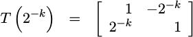This transformation matrix has the unique property that it can be applied to an x and y coordinate vector without requiring any hardware multiplies to calculate the result.

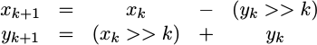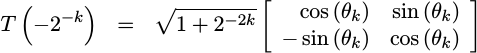
We’ve also discussed how this coordinate transformation can be rearranged to look like a rotation matrix,

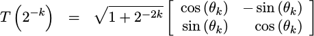where

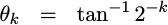Likewise, if you switch the sign of the angle, the rotation is easily reversed. The resulting transform looks almost identical, save for a couple of sign differences,

For this algorithm, we’ll apply a series of CORDIC rotation matrices to our input vector until the y value lies on the x-axis. If you’d like, you can follow along the discussion that follows while looking at the Verilog code for this operation here

The preliminary stage

You may remember from before that the maximum CORDIC rotation is +/- 45 degrees. We’d like to create an algorithm that works for all angles. That means we’re going to need to a preliminary rotation step to bring us to within +/- 45 degrees of the x-axis, as shown in Fig 2.

Fig 2: Pre-rotation results

Fig 3: Pre-rotation to +/- 45 degrees

Unlike the last time, we can’t use the i_phase angle to define this initial rotation, since the phase is something we are trying to calculate. Instead, we’ll use the signs of the initial vector, i_xval, i_yval to determine our pre-rotation coordinate conversion. This leads us to a pre-rotation step that looks like Fig 3.

Notice from the figures that our initial rotation areas are aligned on multiples of ninety degrees. This is a result of starting with the signs of i_xval and i_yval.

You may find that the code for this initial rotation looks very similar to the code we presented in our original CORDIC post. Unlike the last time, this pre-rotation requires adding the (potentially negated) x and y values together to accomplish the rotation.

// First stage, map to within +/- 45 degrees
always @(posedge i_clk)
if (i_ce)
	case({i_xval[IW-1], i_yval[IW-1]})
	2'b01: begin // Rotate by -315 degrees
		xv[0] <=  e_xval - e_yval;
		yv[0] <=  e_xval + e_yval;
		ph[0] <= 19'h70000;
		end
	2'b10: begin // Rotate by -135 degrees
		xv[0] <= -e_xval + e_yval;
		yv[0] <= -e_xval - e_yval;
		ph[0] <= 19'h30000;
		end
	2'b11: begin // Rotate by -225 degrees
		xv[0] <= -e_xval - e_yval;
		yv[0] <=  e_xval - e_yval;
		ph[0] <= 19'h50000;
		end
	// 2'b00:
	default: begin // Rotate by -45 degrees
		xv[0] <=  e_xval + e_yval;
		yv[0] <= -e_xval + e_yval;
		ph[0] <= 19'h10000;
		end
	endcase

That’s the pre-rotation step. We’re now within forty five degrees of the final “correct” answer.

Rotating the vector towards zero

Having accomplished the pre-rotation step, it’s now time for the guts of the algorithm. The algorithm starts out identical to the last time, with a generate statement and a for loop across stages.

genvar	i;
generate for(i=0; i<NSTAGES; i=i+1) begin : TOPOLARloop
	always @(posedge i_clk)

When you get to the actual implementation of the CORDIC rotations themselves, the big difference between this section of code and the previous one is the dependence upon the sign of yv rather than the sign of the remaining phase angle ph. If the sign is negative, apply the CORDIC rotation in the CCW direction, otherwise rotate CW. In both cases, we’ll accumulate the rotation amount in the phase variable, ph.

	if (i_ce)
	begin
		if (yv[i][(WW-1)]) // Below the axis
		begin
			// If the vector is below the x-axis, rotate by
			// the CORDIC angle in a positive direction.
			xv[i+1] <= xv[i] - (yv[i]>>>(i+1));
			yv[i+1] <= yv[i] + (xv[i]>>>(i+1));
			ph[i+1] <= ph[i] - cordic_angle[i];
		end else begin
			// On the other hand, if the vector is above the
			// x-axis, then rotate in the other direction
			xv[i+1] <= xv[i] + (yv[i]>>>(i+1));
			yv[i+1] <= yv[i] - (xv[i]>>>(i+1));
			ph[i+1] <= ph[i] + cordic_angle[i];
		end
	end
end endgenerate

When we are all done, the amount of phase rotation that we’ve applied can be found in ph, while the magnitude of the resulting vector can be found in xv. The y-value, yv, for the final stage should also be zero or nearly so, making it irrelevant. Our next step will be to round this value to the desired number of output bits, and return the result.

Rounding the result

Some time back, we discussed the serious problems that can be associated with truncation. Ever since, I’ve recommended convergent convergent rounding whenever the number of bits in a value needs to be lowered. Therefore, as a last step, we’ll apply convergent rounding to our magnitude value, xv.

assign	pre_mag = xv[NSTAGES] + { {(OW){1'b0} },
			xv[NSTAGES][(WW-OW)],
			{(WW-OW-1){!xv[NSTAGES][WW-OW]}}};

always @(posedge i_clk)
if (i_ce)
begin
	o_mag   <= pre_mag[(WW-1):(WW-OW)];
	o_phase <= ph[NSTAGES];
end

Notice that we didn’t apply any rounding to our phase angle result. That’s because we’ve never dropped bits in the phase angle. Indeed, the number of phase bits has been constant at PW throughout the algorithm.

This is the last of the three differences between today’s development and the CORDIC agorithm we presented last time. At this point, our development is complete. As with the basic CORDIC agorithm, this one will also use a core generator–however the changes necessary to make that core generator–however work were just presented above.

Feel free to check out the core generator as well as the examples of the code it produces.

Conclusion

Now that we’ve gone through and explained the differences between the CORDIC rotation agorithm and this rectangular to polar converter, we’ve now finished presenting the basic uses of the CORDIC algorithm.

While we haven’t discussed the code generator for this rectangular to polar converter, it follows from the discussion above. You can find the completed core generator on github, as part of the CORDIC repository.

If you refer back to Ray Andraka’s paper, Andraka shows several other uses for a basic CORDIC algorithmic approach: arcsine and arccosine generation, calculating hyperbolic trigonometric functions and more. Feel free to do some research should you need algorithms for any of these other functions.

Our development, though, is by no means complete. Our next step in this development will be to build a test bench for these routines. We may even go as far as to connect our sine/cosine generator to an audio amplifier, but we’ll see how the direction works out. Our eventual goal, though, is going to be to use the sine and cosine generation capability of the CORDIC as part of a test bench for the digital filters I’d like to present and demonstrate.