
Spectrograms need Window Functions
If you are going to be doing DSP on an FPGA, chances are you are going to want to know if your DSP is working. That requires being able to visualize what’s going on somehow.
How shall waveforms be visualized?
Perhaps the easiest answer, when dealing with audio rate signals, is not to visualize them at all but just to play the sound into a set of headphones. It’s amazing how good the ear is at picking up sound quality–both good and bad. The only problem is that while ears are good at telling you if there is a problem, they’re not nearly as good for identifying the problem. Worse, from the standpoint of this blog, it’s hard to be communicate subtle differences in sound within an article like this one.
Perhaps the next best answer is to visualize the waveform in time. This works okay enough for some sounds. For example, it’s not that hard to find when certain percussion instruments strike, but there’s often more to percussive instruments than just the striking itself. How, for example, shall a marimba be differentiated from a snare drum or a xylophone for example?
As an example, consider the humpack whale song shown in Fig. 1 below.
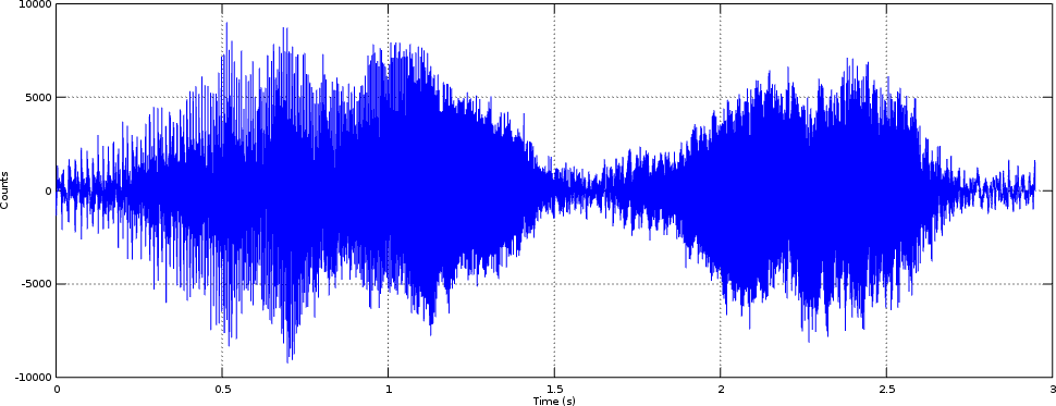 |
Judging from this picture alone, what can you determine? While I’m not trained in whale song, I can see that this whale has spoken twice in this clip, but that’s about it.
Were we examining music, a musician would want to know what notes are being played and when. This is great too, except … not all “middle C”s sound the same. A piano playing a middle C sounds different from a trumpet, from a pipe organ, a clarinet, a flute, etc. This information would need to be able to be visualized somehow as well.
While I’m not a recording studio engineer, I’ve been told that there’s a big difference between studio silence and other types of silence. For example, is your house really quiet when the dishwasher, laundry, and refrigerator are all running? How will you know your recording is good enough that these background noises have been properly removed?
The problem isn’t limited to music, either, nor is it limited to the human hearing range. What about whale song or seismic analysis? Or, for that matter, what about microwave radar analysis? How shall you know if a radar, or even a radar jammer for that matter, is producing the right waveform by looking at it? You can’t listen to it–it’s too wideband, neither will it necessarily “sound” like anything you might recognize. (I’ve known people who have found ways of doing this anyway ….)
As an example of what spectral analysis might show, consider Fig. 2 below, showing the same whale song from Fig. 1 above.
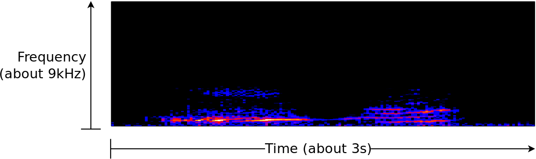 |
In this image, time goes from left to right, and frequency from DC at the bottom to about 9kHz on the vertical axis. From here, you can see that the two whale sounds have very different spectral features. In the first, the whale has emitted a rough tone. In the second, the whale has changed the sound of the tone, and hence you can see the introduction of harmonics. Further, there’s a bit of a sweep to the second tone.
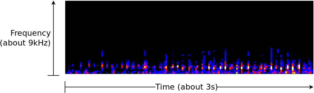
Whales can also emit a series of clicks. Fig. 3 below shows a series of humpack whale clicks–also using the same spectral representation.
 |
Now consider the bowhead whale spectra, shown in Fig. 4 below.
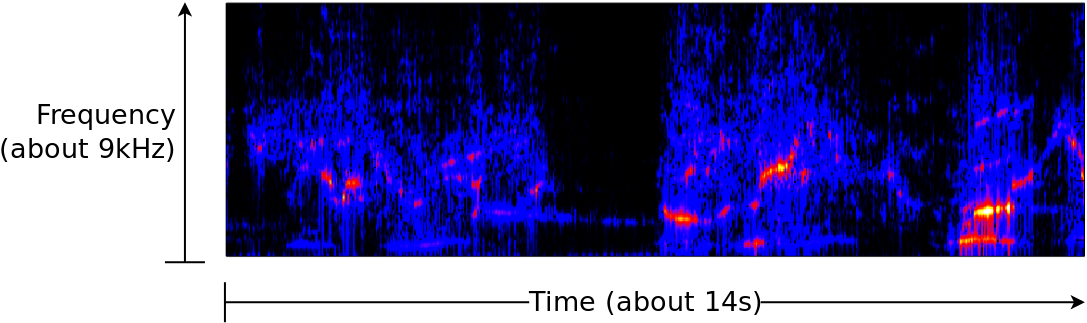 |
From here, you can see that the bowhead has a much higher pitch, and also that there are much larger frequency sweeps.
Would you have been able to see these details without dividing the signal into time and frequency?
No, and that’s the bottom line: you’re going to want to do some type of time-varying spectral analysis when processing signals. The purpose of time-varying spectral analysis is to determine the frequency content of a particular signal, and see how that frequency content changes with time–much like we did with the examples of the whale song above.
Some time ago, we discussed a super cheap way of doing spectral analysis. While this approach can work nicely in some circumstances–such as when examining stationary processes, it’s not a real-time method for the simple reason that part of the algorithm involves dropping data. Sure, it’s useful for debugging, but it’s not very useful for seeing how a signal’s spectral content develops and changes over time.
For all these reasons, let’s take a look today at the traditional way of doing this within an FPGA: windowed FFTs. Before we get there, though, let’s back up and develop the concept of a spectral density.
What is a Power Spectral Density
One of the key purposes of spectral density estimation is to find out where the energy in a signal lies spectrally. For this reason, let’s start back at the beginning and discuss both power and power spectral densities (PSDs).
Let’s start at the top. The voltage drop across a resistor, from Ohm’s law, is given by the product of the current going through the resistor times the resistance of the resistor.
 |
The power
being consumed by this same resistor is given by
 . Hence,
if you know the voltage and the resistance across which it is measured, then
you know the
power to be,
. Hence,
if you know the voltage and the resistance across which it is measured, then
you know the
power to be,
 |
You can use a voltmeter,
or even an analog to digital
converter, to
measure voltage, so let’s work with that. Let’s say we do this and get samples,
![`x[n]`](/img/windowfn/expr-xn.png) , from our A/D
converter.
Power is then related to,
, from our A/D
converter.
Power is then related to,
 |
where the (scale factor) captures the impact of both the
resistor and the sample
rate.
This scale factor is important when converting from
A/D units
representing quantized values to true
power
measured in Watts, but for now we’re going to ignore it so that we can focus on
the algorithms used to separate this energy into separate frequency components.
In other words, now that I’ve noted the existence of this scale factor, I’m
going to drop it entirely from the discussion that follows.
The  term comes from the simple fact that
power is a unit of
average energy per unit of time. If, at every time instant, we get a new
term comes from the simple fact that
power is a unit of
average energy per unit of time. If, at every time instant, we get a new
![`|x[n]|^2`](/img/windowfn/expr-abs-x-n-squared.png) value,
then our
“power”
would appear to increase even if
were constant and all these values were the same. Indeed,
is a measure of energy, not
power.
Hold on to that thought, though, we’ll come back to it in a moment.
value,
then our
“power”
would appear to increase even if
were constant and all these values were the same. Indeed,
is a measure of energy, not
power.
Hold on to that thought, though, we’ll come back to it in a moment.
For now, let’s increase our averaging interval until we are averaging across all time. This then becomes the total power in our signal, and it allows us to talk about and reason about power that might change over time while still having a measure of total power.
 |
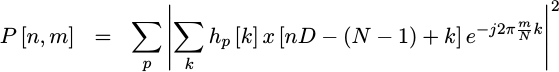
Now that we have this expression for the power measured by an A/D, we’d like to know how much of this power was captured in a spectrally significant ways Can we split this summation over frequency instead of time? Ideally, we’d like something that both measures our total power, yet also isolates that power by frequency. This is the purpose of the Power Spectral Density Function (PSD).
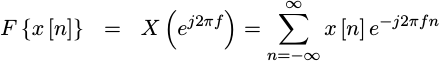
How shall we get there? Simple, let’s take a Fourier
transform of the
elements of this summation. We’ll start by letting
![`F{x[n]}`](/img/windowfn/expr-Fx.png) represent the
Fourier transform
of our input.
represent the
Fourier transform
of our input.
 |
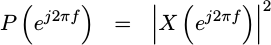
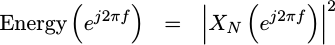
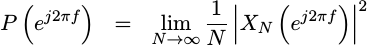
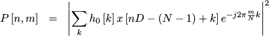
The PSD
of the signal,  is then just the square of this value.
 |
This is where we run into our first problem. What happened to the
term?
The answer is, we got sloppy and dropped it. Worse, our
Fourier transform
summation above doesn’t converge when we apply it either to a constant signal
or a constantly varying signal. No, we’ll need to back up and rework this.
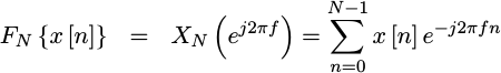
In particular, we’ll need to be explicit about the limits in our
Fourier transform.
 |
If we insist that
 be finite, we’ll know that the transform converges.
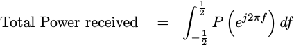
We can now apply Parseval’s theorem, knowing that the integral of this |X(f)|^2 function should give us back our total energy, and that energy averaged over time is power.
 |
Therefore,
 |
and
 |
 |
This leads to the first important rule of PSD estimation: No power should be accidentally gained or lost during our analysis. Our goal must be to preserve this total received power measurement.
What happens, though, if we only look at a band of frequencies instead?
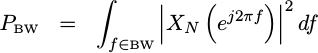 |
 |
We’d then have an estimate of how much power lied between these frequencies.
If you then take the limit of this power measurement as the bandwidth goes to zero, you’ll get a PSD.
Sadly, this infinite limit over time makes the
PSD
difficult to work with, if for no other reason than it’s impossible to sample
a signal for all time in order to estimate its
PSD.
So, what if we didn’t take the limit as
 ?
We’d then have an energy measurement,
rather than a power
measurement. Not only that, but our
measurements suddenly get a lot more practical to work with.
?
We’d then have an energy measurement,
rather than a power
measurement. Not only that, but our
measurements suddenly get a lot more practical to work with.
For example, if our signal were limited to
samples rather than an
infinite number, then we could use a discrete time Fourier transform
(DTFT) instead.
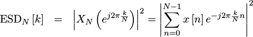 |
Now we’re getting somewhere, right? This is something I can calculate, and a value I can use!
Only … it’s not that useful.
The problem has to do with our limits. Our original signal was unlimited in time. We then arbitrarily forced limits in time upon it. This will cause spectral energy to spill from one frequency region to another. The solution to this problem is to use a spectral taper, sometimes called a window function.
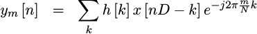
The Short-Time Fourier Transform
There have been a lot of discussions regarding how to ideally decompose a signal into time and frequency. One reference I’ve enjoyed has been Cohen’s book on Time-Frequency Analysis. It does a nice job of providing a good overview of the topic. That said, the first thing Cohen does is to reject the Short Time Fourier Transform based methods for other more generic quadratic methods–methods that don’t even preserve the concept of energy in the first place. Most of the methods he discusses will produce both positive and negative “energy” estimates.
 |
Negative energy? That doesn’t make any sense. Sorry, but I’ll need another approach.
The next important spectral estimation reference is Scharf, Friedlander and Mullis’ paper, Time-varying spectrum estimators, which works out the form of the ideal spectral estimator from first principles. If you are interested in this topic, I would highly recommend this paper to you before any other references. By insisting that energy should always be non-negative, Scharf, et.al., are able to drastically limit the kind of spectral estimation algorithms that need to be examined. By further limiting the set of all possible time-varying spectral estimators to only those which preserve our understanding of both time and frequency, they are able to limit the set of spectral estimators to the set of estimator’s generated by multiple-taper windows.
 |
I’d like to add to this discussion the proof that, if you want the maximum time-frequency resolution, then nothing beats a single taper representation.
 |
There’s a nice proof available for this, so it’s something we may need to come back to later. Getting there, however, will take some work–so let’s just look at how to implement a single taper estimate in the first place. For that, we want to look into how to implement the single-taper implementation known as a window function.
Here’s the basic idea of how this works:
-
We’ll break a stream of incoming data into chunks, each the size of one FFT and each separated by
 samples.
If
samples.
If  then there will necessarily be some amount of overlap between
these various chunks.
then there will necessarily be some amount of overlap between
these various chunks.![`CHUNK[nD] = x[nD-(N-1)], ... x[nD]`](/img/windowfn/eqn-data-chunk.png)
We’ll come back to this in a moment, but for now remember that 50% overlap is easy to build and (often) sufficient for most purposes.
-
We’ll then apply our window function to each chunk of data.
![`WINDOWED[nD] = h[N-1]x[nD-(N-1)], ... h[0]x[nD]`](/img/windowfn/eqn-windowed-raw.png)
As a notational simplification, if we insist that
![`h[k] = 0`](/img/windowfn/eqn-hk-eq-zero.png) for
for
 or
or
 ,
then we might just refer to
,
then we might just refer to
![`h[k]x[nD-k]`](/img/windowfn/expr-hk-xnD-k.png) .
.![`WINDOWED[nD] = ... h[k]x[nD-k] ...`](/img/windowfn/eqn-windowed-data.png)
You might also note that this window function is starting to look like a digital filter. That’s because it is a digital FIR filter. Indeed, one of Allen’s observations is that a windowed Fourier transform produces a series of filtered, downconverted, and downsampled outputs.
-
As a final step, we’ll apply an FFT to that windowed chunk of data, and report and record the results.
 |
To do this in a useful fashion, there are a couple of basic criteria you’ll need:
-
The window function, h[k], needs to be a lowpass filter with a strong stopband rejection.
While they may not be optimal, most of your traditional window functions meet this criteria: Hann, Blackman, Hamming, Bartlett, etc.
-
To satisfy the requirements of the Nyquist sampling theorem, it is important that the step size be related to the cutoff frequency of the lowpass filter. In general, this means that
must be less than or equal to
 .
.This choice is actually related to the window function design. What should the cutoff frequency of the window function be? One might argue that the ideal window function would isolate various signal frequency components to their nearest bins. For example, if a tone were anywhere within a frequency bin, it should then create a response in that bin and that bin only. Such a window would be a lowpass filter with a cutoff frequency of
 , an
infinitesimal transition
band, and an infinite
stopband rejection.
, an
infinitesimal transition
band, and an infinite
stopband rejection.If you’ve studied digital filter design at all, you’d recognize this filter requirement as the first filter that gets studied–and then rejected because it is unrealizable due to its infinite length.
Better windows exist.
If we instead compromised and allowed energy to spill a little bit from one bin to the next, then we might allow energy to spill into the two FFT bins on either side of any bin of interest. As a tone moved from one bin to the next, the decomposed spectral energy should also transition from one bin to the next. This requires a filter with a stopband region starting at
,
but here’s the key criteria:
we don’t need a passband.
The entire band of interest could be within the
transition band
of this filter. That makes the filter realizable.It also means we want to sample the output at twice this rate in order to avoid any aliasing, which then brings us back to a minimum 50% overlap.
 |
While zero padding in time can help to create the illusion of better
frequency resolution, you can also increase your overlap amount to create
a similar illusion of better time resolution. In this case, the right
answer depends upon the cutoff frequency of your
window function,
and the sample rate required to avoid losing information. As an example,
when using a Hann window,
you might want to set
 to create a 75%
overlap. This will keep your spectral data from suffering any
aliasing artifacts.
to create a 75%
overlap. This will keep your spectral data from suffering any
aliasing artifacts.
The problem with using a greater overlap is simple: you end up with more
data to process. That is, if you have an incoming sample rate of
 , and
you set the decimation factor to
, and
you set the decimation factor to
 , you’ll now have
a data rate that you need to process that’s twice as fast, or
, you’ll now have
a data rate that you need to process that’s twice as fast, or
 . If you set
on the other hand,
you now have to process a data stream at a rate of
. If you set
on the other hand,
you now have to process a data stream at a rate of
 , four times
as fast as the original data stream. While you can do this to avoid the
aliasing
problems associated with the
Hann window,
window,
there are better
window functions
with tighter cutoffs.
, four times
as fast as the original data stream. While you can do this to avoid the
aliasing
problems associated with the
Hann window,
window,
there are better
window functions
with tighter cutoffs.
Still, the Hann window will be a nice one to work with when using the algorithm that follows. Indeed, it is one of my favorites among the classic window functions for the simple reason that it is fairly easy to analyze.
-
The important part of window function selection is to make sure that whatever window you choose, it should preserve the conservation of energy principle that we started with. That is, when we are done, we’ll want to make certain that,
![`PTOTAL = LIMIT N-> INFTY (1/N) |ym[n]|^2`](/img/windowfn/eqn-final-ptotal.png)
This is one of the drawbacks of most of your traditional window functions, to include my favorite Hann window. Most of these functions will over or undercount certain spectral or temporal energy. The solution would be to use a root-Nyquist filter, of which Root-Raised cosine filters are the best known subset despite their poor out-of-band performance.
-
At this point, if we have a lowpass windowing function, together with better than Nyquist sampling, together with our conservation of energy requirement, we know that our window function will localize the energy in the incoming signal to a particular band. Even better, we can take summations across multiple band outputs to estimate the amount of energy limited by those spectral bands.
![hat{P}BS(m/N) = SUM^{k=-BW/2}^{BW/2} |ym+k[n]|^2](/img/windowfn/eqn-psdhat-sum.png) |
This was one of our success criteria, and it looks like we’ve achieved it.
It’s actually better than that. Not only can we localize energy spectrally, but we can also locate energy in time. Hence, we have a time–varying spectral energy estimator as desired.
Pretty cool, huh?
Curiously, the conservation of energy criteria together with the lowpass filter cutoff criteria are sufficient for the transform to be invertible. See Allen or Crochiere for more information on this.
For now, the question I would like to focus on today is how the basic Windowed FFT structure should be implemented within an FPGA.
Implementation Overview
Let’s start out with just a simple and general overview of how a spectral analysis design might work.
As with any data processing design, the data processing is typically done within some tight data loop, where the first step is to grab data.
	while(!done) {
		// Get some number of data samples
		get_adc_data(buffer);
If the data isn’t (yet) ready, the easy answer is to stall within this function until a sufficient amount of data becomes ready. Once a buffer is ready, then it can be returned and further processed.
For the sake of discussion today, we’ll assume this buffer is a buffer of
double while working in C++. Of course, we’ll have to change that to
fixed point
once we switch to Verilog, but I’m likely to gloss over any difference
in details between the two–even though the difference between
floating and
fixed point
formats is far from inconsequential.
Once we have our data samples, we’ll apply our window function as described above and as we’ll discuss further below.
		// Apply a window function
		apply_window(buffer);
The result of applying a window function to our new data is a buffer of data, sized to the size of our FFT, which we then send directly into the FFT. For now, let’s assume the incoming data buffer size is the same as the FFT size–and fix this in a second design attempt further down.
		// Take an FFT of the results
		fft(FFTSIZE, buffer);
We now have the results of an FFT, only we can’t plot them. FFTs return complex data: there’s both real and imaginary components. There’s no easy way to plot complex data like that. However, as described above, we don’t really want complex data: we want the absolute value squared of our data. Therefore, we want to replace our data with its absolute value squared. Optionally, we could also convert the result to Decibels at this time as well. (Note that this transformation is non-linear, so you may wish to keep a copy of the original signal around when you do this.)
		// Calculate absolute magnitude squared
		// of the complex results
		for(k=0; k< FFTSIZE/2; k++) {
			buffer[k]  = buffer[2*k  ] * buffer[2*k  ];
			buffer[k] += buffer[2*k+1] * buffer[2*k+1];

			// Optionally, convert to decibels
			// buffer[k] = 20 * log(buffer[k]) / log(10.0);
		}
You might notice that I’m not being consistent here: I’m mixing real data and
complex
data together. Were the original data set real, the
FFT might return the
DC component in buffer[0] and the N/2 component in buffer[1]. In that
case, it would be inappropriate to mix these two components together.
Likewise, if the original data were
complex that were then
Fourier transformed,
you might now want to apply an FFT
shift to place the DC value in the center of the band. I’m just glossing over
these details for now because it’s not the focus of what
I really want to discuss–the implementation of the
window function itself.
The next step, required prior to displaying any spectral energy data, is to scale it to what the screen can display. For a graph plot, this might also mean adjusting the vertical axis so things can fit. For rastered time varying energy spectral data, you’ll need to scale the data so that it then represents an index into a color map–something we can discuss again in another article.
		// Possibly scale the results
		if (OPTIONALLY_SCALE)
			scale(buffer);
Finally, at this point, we can now plot our buffer and repeat this whole process for the next incoming data buffer.
		// Plot the result
		plot(buffer);
	}
If you are curious what these steps might look like in Verilog, check out the main verilog file from this FFT raster demonstration. The biggest difference is that FPGAs operate on live data streams rather than data blocks–but the concepts remain the same.
So now that we’ve looked over the context of how a window function might fit into a larger algorithm, how should it be implemented? It’s really simple: we’d take our data, and multiply each sample of it by the window function before returning it.
double	m_window[FFTSIZE];

void	apply_window(double *data) {
	for(k=0; k<FFTSIZE; k++)
		data[k] = m_window[k] * data[k];
}
If we could keep the algorithm that simple, then it would also be quite easy to implement in Verilog. All we’d need to do would be to multiply every incoming sample by the window’s coefficient to create an outgoing sample.
always @(posedge i_clk)
if (i_ce) // For every incoming sample ...
begin
	// 1. Calculate a windowed outgoing sample
	o_sample <= cmem[tidx] * i_sample;

	// 2. Mark the following outgoing sample as valid
	o_ce <= 1;

	// 3. Increment the index into our coeffficient table
	tidx <= tidx + 1;

	// 4. Mark the first outgoing sample
	o_frame <= (tidx == 0);

end else begin
	// Clear the outgoing valid signal, making certain it's
	// only ever high for one cycle.
	o_ce <= 0;
end
This rudimentary implementation has a couple of problems, however. One problem is that you can’t read from block RAM and use the result on the same cycle. A second more fundamental problem is the fact that this window function implementation doesn’t handle any overlap.
So let’s back up and discuss how we might handle overlap for a moment.
At a minimum, we need to keep track of the last half FFT’s worth of incoming data. That will require a buffer. Practically, we have to keep track of more than just the last half of the FFT’s incoming data, since it will be hard to capture the next half FFT’s worth of data without destroying the data we still need to use along the way.
Therefore, let’s start out with a buffer the size of a full FFT, and an index into where the most recent data is within that buffer. This will allow us to use one half of the buffer, while reading new data into the second half.
int	m_loc = 0;		// Index into our buffer
double	m_window[FFTSIZE];	// Window function coefficients
double	m_data[FFTSIZE;		// Data buffer
Now, every time we get N/2 samples, herein noted as FFTSIZE/2, we’ll call
our apply_window() function. This function will consume FFTSIZE/2 samples,
and then produce FFTSIZE windowed samples as outputs.
//
// FFTSIZE/2 data comes in, filling the first FFTSIZE/2 samples of the
// given buffer.  The input buffer's size, however, must be FFTSIZE in
// length to handle the returned window data
//
void	apply_window(double *input) {
	int	pos;
	double	*ptr, *tap, *inp, *outp;
The first task of this function will be to copy the new data into the oldest position in our buffer. If we keep the new data location aligned with the overlap, then this copy can be done quite simply.
	// Add the input to our buffers ...
	ptr = &m_data[m_loc];
	inp = input;
	for(pos=0; pos<FFTSIZE/2; pos++)
		*ptr++ = *inp++;
If the new data amount wasn’t a factor of the FFT size, we would’ve then also needed to check for overflowing the end of our buffer in the middle of the loop. With an exact 50% overlap, though, we can skip that check.
We’ll then advance the data location pointer by a half FFT length, and force it to stay within one FFT’s size.
	m_loc += FFTSIZE / 2;
	m_loc &= (FFTSIZE-1);
We now have a full
FFT’s
worth of data to apply our
window to. This data
will either be the m_data buffer itself, or the two halves of the m_data
buffer in reversed order. That means we’d need to apply the
window one half at a time.
So, let’s start with the first half–the half that starts out with the data left in the buffer from the last window function invocation.
	// Apply the filter to generate a block for FFT'ing
	ptr = &m_data[m_loc];
	outp = input;
	tap = m_window;
	for(pos=0; pos<FFTSIZE/2; pos++)
		*outp++ = *ptr++ * *tap++;
Again, because we’ve guaranteed that m_loc is either 0 or FFTSIZE/2, we
don’t need to check for pointer boundaries within this loop.
To handle the next half, we’ll need to update our data pointer. This will either leave it the same, or set it to the first half. We can then loop over the second half.
	ptr = &m_data[m_loc ^ (FFTSIZE/2)]
	for(pos=0; pos<FFTSIZE; pos++)
		*outp++ = *ptr++ * *tap++;
}
Voila! We’ve just accomplished a window function while handling overlap.
How would we do this from Verilog?
Well, the first difference is that we’ll always have data coming in–whether or not we’re ready for it. That data will need to be stored into our buffer.
	initial	dwidx = 0;	// Data write index
	always @(posedge i_clk)
	if (i_ce)
	begin
		dmem[dwidx] <= i_sample;
		dwidx <= dwidx + 1;
	end
The next big problem will be how to handle the data rate change–data comes into
our algorithm at one rate, and it must go out at twice that rate. To handle
that, I’m going to create two “clock enable” inputs: i_ce, for when valid
data comes in, and i_alt_ce, to describe the pipeline between valid data
samples. Our rule will be that i_alt_ce must be high once, and only once,
between every pair of clocks having i_ce high. That way we have a data
stream clocking signal handling both clocks. You can see an example of what
this might look like in Fig. 5 for an 8-point
FFT.
 |
Hence, for every incoming sample, i_ce, we’ll create an outgoing clock
enable. Likewise for every incoming i_alt_ce, we’ll also create an outgoing
clock enable. Further, at the beginning of every outgoing burst we’ll set an
o_frame signal to indicate the first clock cycle in the frame.
This alternate data valid signal, i_alt_ce, could easily be set to a one-clock
delayed version of i_ce. I’ve chosen not to do that here, lest the output
need to go through a “slow” DSP processing engine that depends upon a
minimum number of idle clocks between outgoing samples.
You’ll also notice from Fig. 5 that the output starts with the first
four samples from the last FFT,
followed by the new four samples. In the picture, these last four samples
are listed as WX0 through WX3, whereas the new ones are listed as
wD0 through wD3. In the second block of data, those same samples are listed
as WD0 through WD3–since they’ve now been multiplied by the second half
of the window function.
Having two clock enable signals, whether i_ce or i_alt_ce, will mean that
we need to update our internal indexes anytime either is true. This would
lead to an indexing algorithm looking (almost) like:
	always @(posedge i_clk)
	if (i_ce || i_alt_ce)
	begin
		tidx <= tidx + 1;	// Coefficient index
		didx <= didx + 1;	// Data index
	end
That would be the first clock of our processing. Once we know which data to read and what memory to read it from, we’d then read from the two memories–both data and coefficient.
	always @(posedge i_clk)
	begin
		data <= dmem[didx];
		tap  <= cmem[tidx];
	end
On the next clock, now that we have both of these values, we can multiply them together to get the window product we want to create.
	always @(posedge i_clk)
		o_sample <= data * tap;
We could then use a simple shift register to determine when an outgoing
sample should be valid. We’ll use d_ce to represent when our data is valid,
p_ce to represent when our product is valid, and o_ce to represent when
the outgoing sample is valid.
	always @(posedge i_clk)
		{ o_ce, p_ce, d_ce } <= { p_ce, d_ce, (i_ce || i_alt_ce) };
Sounds easy enough, right? Fig. 6 shows how some of these respective CE signals might relate.
 |
Not quite.
The first problem is the data index. While it should go through the data
from 0...N-1 the first time through, we want to go through
samples N/2...N-1, 0 ... N/2-1 the second time through. We’ll then want
to alternate between these two index sequences.
How shall we know which sequence to use at any given time? For that, we can
use the data writing index. On the last sample of any window set, following
the last i_ce in the set, the data write index will then be set to write
a new sample to the next buffer.
	always @(posedge i_clk)
	if ((i_alt_ce)&&(dwidx[LGNFFT-2:0]==0))
	begin
We can then use this write index as an indication that the data sample read index should be adjusted.
		// Restart on the first point of the next FFT
		didx[LGNFFT-2:0] <= 0;
		// Maintain the top bit, so as to keep
		// the overlap working properly
		didx[LGNFFT-1] <= dwidx[LGNFFT-1];
For all other samples, though, we’ll simply increment the data read index as before.
	end else if ((i_ce)||(i_alt_ce))
		// Process the next point in this FFT
		didx <= didx + 1'b1;
Indeed, our process really shouldn’t be any more complicated than that.
Window Function Details
With all that background behind us, let’s turn our attention to the detailed design and implementation of this window function.
 |
We’ve gone over most of the ports already, so the port list of this function shouldn’t be too surprising.
The one item we haven’t discussed yet is a mechanism for updating the
coefficients of the window function. In this case, I’ve chosen to use
the i_tap_wr interface to indicate that a new coefficient is available
in i_tap to write into the filter. I suppose I could have used a more
general purpose block RAM interface, but I’ve chosen this interface to be
consistent with those faster filters that can’t handle the block RAM interface.
We’ve discussed the rest of the ports above: i_clk and i_reset should
be self explanatory. i_ce will be true for every incoming data value, and
i_alt_ce will need to be true once between every pair of i_ce values as
shown in Figs. 5 and 6 above. When the output is ready, o_ce will be
asserted and the sample will be placed into o_sample. We’ll also note
the first sample in any block by setting o_frame.
`default_nettype	none
//
module	windowfn(i_clk, i_reset, i_tap_wr, i_tap,
		i_ce, i_sample, i_alt_ce,
		o_frame, o_ce, o_sample);
We’ll allow for an input width of IW bits, an outgoing width of OW bits,
and a coefficient width of TW bits. (Sorry, but I consider filter
coefficients to be taps, and get my notation confused. The term tap
more appropriately describes the structure of the filter rather than the
coefficients themselves. Still, you’ll find tidx referencing a coefficient
index below, and TW referencing the bit-width of coefficients here.)
The default implementation will also support an
FFT size of 2^LGNFFT, or
16 samples.
parameter IW=16, OW=16, TW=16, LGNFFT = 4;Why is the default so short? It makes coverage easier to check. That’s all.
If you want to be able to update the coefficients on the fly, then you’ll want
to leave OPT_FIXED_TAPS at zero. Likewise, if you want to load the
initial coefficients from a file, we’ll offer an INITIAL_COEFFS filename
for that purpose.
	parameter	[0:0]	OPT_FIXED_TAPS = 1'b0;
	parameter		INITIAL_COEFFS = "";
The next optional parameter, OPT_TLAST_FRAME deserves some more discussion.
parameter [0:0] OPT_TLAST_FRAME = 1'b0;If you want to convert this design from my own signaling scheme into an
AXI-stream based signaling protocol, you’ll run into a problem with TLAST.
Yes, most of the conversion is easy.
For example, a small FIFO on the back end can handle stopping the window
on any back pressure.
Just be careful to update the fill of that FIFO
based upon the data going into the front end. The problem lies with the
o_frame output. I’ve chosen to set o_frame on the first sample of any
data set. AXI Stream likes a TLAST value, where TLAST would be true on
the last item in any data set. Hence the parameter, OPT_TLAST_FRAME.
If OPT_TLAST_FRAME is set, then o_frame will be set on the last sample
in any FFT frame–overriding my
favorite behavior.
The rest of the port declarations are fairly unremarkable.
	localparam	AW=IW+TW;
	//
	input	wire			i_clk, i_reset;
	//
	input	wire			i_tap_wr;
	input	wire	[(TW-1):0]	i_tap;
	//
	input	wire			i_ce;
	input	wire	[(IW-1):0]	i_sample;
	input	wire			i_alt_ce;
	//
	output	reg			o_frame, o_ce;
	output	reg	[(OW-1):0]	o_sample;
As I mentioned above, we’ll need two memories: one for the coefficients, and one for the FFT data itself so that we can maintain proper overlapping.
	reg	[(TW-1):0]	cmem	[0:(1<<LGNFFT)-1];
	reg	[(IW-1):0]	dmem	[0:(1<<LGNFFT)-1];
The coefficients themselves can be loaded from a basic $readmemh function
call.
	//
	// LOAD THE TAPS
	//
	wire	[LGNFFT-1:0]	tapwidx;
	generate if (OPT_FIXED_TAPS)
	begin : SET_FIXED_TAPS

		initial	$readmemh(INITIAL_COEFFS, cmem);

		// ...
	end else begin : DYNAMICALLY_SET_TAPS
The more interesting case is the dynamic handling.
In this case, we’ll need a coefficient writing index. Then, on any write to the coefficient memory, we’ll write to the value at this index and increment it by one.
		// Coef memory write index
		reg	[(LGNFFT-1):0]	r_tapwidx;

		initial	r_tapwidx = 0;
		always @(posedge i_clk)
		if(i_reset)
			r_tapwidx <= 0;
		else if (i_tap_wr)
			r_tapwidx <= r_tapwidx + 1'b1;

		if (INITIAL_COEFFS != 0)
			initial $readmemh(INITIAL_COEFFS, cmem);
		always @(posedge i_clk)
		if (i_tap_wr)
			cmem[r_tapwidx] <= i_tap;

		assign	tapwidx = r_tapwidx;
	end endgenerate
From here, let’s work our way through the algorithm clock by clock in the pipeline.
Data is available on clock zero. We’ll need to simply write this to our data memory and increment the pointer.
	initial	dwidx = 0;
	always @(posedge i_clk)
	if (i_reset)
		dwidx <= 0;
	else if (i_ce)
		dwidx <= dwidx + 1'b1;

	always @(posedge i_clk)
	if (i_ce)
		dmem[dwidx] <= i_sample;
I’m also going to suppress the first block of
FFT data.
This would be the block prior to where a full
FFT’s worth
of data is available. Hence, on the first_block, I’ll set a flag noting
that fact, and I’ll then clear it later once we get to the last coefficient
index associated with processing that block.
	initial	first_block = 1'b1;
	always @(posedge i_clk)
	if (i_reset)
		first_block <= 1'b1;
	else if ((i_alt_ce)&&(&tidx)&&(dwidx==0))
		first_block <= 1'b0;
The next thing I want to keep track of is the top of the block. That is,
I want a signal set prior to the first data element in any block, that I can
then use as an indication to reset things as part of the next run through any
data. We’ll call this signal top_of_block. We’ll set it when we get the
i_alt_ce signal just prior to writing the first data value.
	initial	top_of_block = 1'b0;
	always @(posedge i_clk)
	if (i_reset)
		top_of_block <= 1'b0;
	else if (i_alt_ce)
		top_of_block <= (&tidx)&&((!first_block)||(dwidx==0));
	else if (i_ce)
		top_of_block <= 1'b0;
Later on, we’ll dig into how to go about verifying this IP core. In general,
my rule is that anything with a multiply within it cannot be formally verified.
But I’d like to pause here and note that neither the first_block flag,
nor the top_of_block flags above involve any multiplies. Neither did I get
them right the first time I wrote this algorithm. My point is simply this: just
because you can’t use formal methods to verify all of the functionality of an
IP core, doesn’t mean that you can’t use them at all. For now, just think
about how much of the logic below can be easily verified formally, and how
much we’d need to verify using other methods. I think you’ll find as we walk
through this implementation that the majority of it can be nicely verified
formally before you even fire up your simulator.
Let’s now turn our attention to the data and coefficient memory indices. As we noted above, it takes a clock to read from a memory. Therefore, these indices need to be available and ready before the first sample arrives. In general, the indices will need to keep pace with the incoming samples, and be synchronized with that same clock zero stage of the pipeline.
The data (read) index is the strange one. This is the one that increments all except for the top bit. The top bit repeats itself between FFTs in order to implement the 50% overlap we’ve asked for.
	initial	didx = 0;
	always @(posedge i_clk)
	if (i_reset)
		didx <= 0;
	else if ((i_alt_ce)&&(dwidx[LGNFFT-2:0]==0))
	begin
		// Restart on the first point of the next FFT
		didx[LGNFFT-2:0] <= 0;
		// Maintain the top bit, so as to keep
		// the overlap working properly
		didx[LGNFFT-1] <= dwidx[LGNFFT-1];
	end else if ((i_ce)||(i_alt_ce))
		// Process the next point in this FFT
		didx <= didx + 1'b1;
When it comes to the coefficient index, all but the top bit of that index will match the data index.
	always @(*)
		tidx[LGNFFT-2:0] = didx[LGNFFT-2:0];
At one time when building this design, I had a second counter for the tidx
coefficient index. One counter was for didx, and a second one for tidx.
Then, when verifying the two, I discovered the bottom LGNFFT-1 bits needed
to be identical. Why then maintain two counters? Hence the combinatorial
expression above.
The top bit of the coefficient index, however, takes some more work. It
follows the same pattern as didx, with the exception that we reset the
top bit at the beginning of any run.
	initial	tidx[LGNFFT-1] = 0;
	always @(posedge i_clk)
	if (i_reset)
		tidx[LGNFFT-1] <= 0;
	else if ((i_alt_ce)&&(dwidx[LGNFFT-2:0]==0))
	begin
		// Restart the counter for the first point
		// of the next FFT.
		tidx[LGNFFT-1] <= 0;
	end else if ((i_ce)||(i_alt_ce))
	begin
To maintain the top bit function, it needs to be set to the carry from all of the lower bits when incrementing.
		if (&tidx[LGNFFT-2:0])
			tidx[LGNFFT-1] <= !tidx[LGNFFT-1];
	end
The next counter, frame_count, is kind of a misnomer. It counts down
three clocks from the beginning of a frame–rather than frames themselves.
Indeed, this is really a pipeline counter. It counts the stages going
through the pipeline after we receive the element that’s going to turn on
the o_frame flag once it gets through the pipeline.
	initial	frame_count = 0;
	always @(posedge i_clk)
	if (i_reset)
		frame_count <= 0;
	else if (OPT_TLAST_FRAME && i_alt_ce && (&tidx)&& !first_block)
		frame_count <= 3;
	else if (!OPT_TLAST_FRAME && (i_ce)&&(top_of_block)&&(!first_block))
		frame_count <= 3;
	else if (frame_count != 0)
		frame_count <= frame_count - 1'b1;
We’ll discuss this more later when we get to the o_frame value below.
Finally, as the last step for this pipeline stage, let’s keep track of when
data values and product results are valid within our pipeline using d_ce
(for data) and p_ce (for the product results).
	initial	{ p_ce, d_ce } = 2'h0;
	always @(posedge i_clk)
	if (i_reset)
		{ p_ce, d_ce } <= 2'h0;
	else
		{ p_ce, d_ce } <= { d_ce, (!first_block)&&((i_ce)||(i_alt_ce))};
That’s it for the first clock, or rather the first pipeline stage of the algorithm.
For the next stage, we’ll want to read the data and coefficient from memory.
	initial	data = 0;
	initial	tap = 0;
	always @(posedge i_clk)
	begin
		data <= dmem[didx];
		tap  <= cmem[tidx];
	end
Remember, because this is block RAM we are reading from, we need to be careful that we don’t do anything more than simply read from it.
Once the block RAM values are ready, we can multiply the two of them together.
	always @(posedge i_clk)
		product <= data * tap;
As before with the block RAM, you’ll want to be careful not to do anything more than a single multiply, or possibly a multiply with a clock enable, in order to insure the DSP will be properly inferred.
Only, if you look through the actual logic for this component, you’ll see something that looks quite a bit different.
	// Multiply the two values together
`ifdef	FORMAL
	// We'll implement an abstract multiply below--just to make sure the
	// timing is right.
`else
	always @(posedge i_clk)
		product <= data * tap;
`endif
Why the difference?
Because formal methods can’t handle multiplies very well. There are just
too many possibilities for the formal engine to check. Therefore, we’ll let
the formal tool generate whatever product value it wants when using formal
methods–subject to only a small number of pipeline verification criteria.
That’ll get us around the problem with the multiply. More on that when we get to the formal methods section below.
That brings us to the last stage of the pipeline–what I call clock #3.
Now that we have our product, all that remains is to set the outgoing
indicators, o_ce, o_frame, and the outgoing sample, o_sample.
The first, o_ce, simply notes when the outgoing data is valid. It will be
valid one clock after the product, allowing us to register the result of the
product.
	initial	o_ce = 0;
	always @(posedge i_clk)
	if (i_reset)
		o_ce <= 0;
	else
		o_ce <= p_ce;
The frame signal, o_frame, is only a touch different. This is the signal that
marks frame boundaries. In general, it will be true on the first sample of
any frame. I can use the frame_count counter, generated above from the
first sample at the top of the frame, or if OPT_TLAST_FRAME is set from
the last sample at the bottom of the frame, to generate this signal.
	initial	o_frame = 1'b0;
	always @(posedge i_clk)
	if (i_reset)
		o_frame <= 1'b0;
	else if (frame_count == 2)
		o_frame <= 1'b1;
	else
		o_frame <= 1'b0;
The last step in the algorithm is to set the outgoing sample.
	initial	o_sample = 0;
	always @(posedge i_clk)
	if (i_reset)
		o_sample <= 0;
	else if (p_ce)
		o_sample <= product;
For the purpose of this article, I’ve kept this final output sample logic
simple, although in the actual algorithm
I rounded it to the output
bit width (OW) instead. This is just a touch cleaner to examine and discuss,
although in practice that rounding operation is
pretty important.
Cover Checks
As we get into verification, let me ask you, where would you start?
You could start with a simple verilog test bench, or even a more complex C++ test bench integrating all of the stages of your FFT together. I chose to do something simpler instead. I started with a simple formal cover statement.
	reg	cvr_second_frame;

	initial	cvr_second_frame = 1'b0;
	always @(posedge i_clk)
	if ((o_ce)&&(o_frame))
		cvr_second_frame <= 1'b1;

	always @(posedge i_clk)
		cover((o_ce)&&(o_frame)&&(cvr_second_frame));
Presenting it here, however, feels a bit out of order. Normally, I group all my cover statements at the end of the design file. Presenting cover here makes it more challenging to compare my draft blog article against the original Verilog file to make sure the two remain in sync.
Chronologically, however, I started verifying this core using cover.
From just this cover statement above, I could easily get a trace from my design. Of course, the first trace looked horrible, and none of the logic matched, but it was still a good place to start from.
The next step that I’ve found useful for a lot of DSP algorithms is to create a counter to capture the current phase of the processing. Where are we, for example, within a block? I can then hang assertions and/or assumptions on this counter if necessary.
For this design, I called this backbone counter, f_phase.
	initial	f_phase = 0;
	always @(posedge i_clk)
	if (i_reset)
	begin
		f_phase <= 0;
	end else if ((i_ce)&&(top_of_block))
		f_phase[LGNFFT-1:0] <= 1;
	else if ((i_ce)||(i_alt_ce))
		f_phase <= f_phase + 1;
This forms the backbone, or the spine of the formal proof.
To see how this works, consider how I can now make assumptions about the
relationship between the i_ce and i_alt_ce signals.
After i_ce, f_phase will be odd and so f_phase[0] will be set. No
more i_ce’s can then follow, until after we’ve an i_alt_ce.
	always @(posedge i_clk)
	if (f_phase[0])
		assume(!i_ce);
I can say the same thing about i_alt_ce and !f_phase[0].
	always @(posedge i_clk)
	if (!f_phase[0])
		assume(!i_alt_ce);
That’s all it takes to get a trace.
 |
From that trace, I can look over the various signals and adjust them as necessary until things look right. At that point, the logic should be starting to work. The next step is to pin down the various signals in the design using assertions, so that we’ll know that the signals within our design will always work this way.
Even better, if we ever make a wrong assertion at this point, we know it should
fail within however many steps it took to generate the cover() trace above
(52). That limits our maximum formal depth. Once I finished with
induction,
though, I managed to get the minimum depth down to four steps. At less than
a second, the proof is pretty quick too.
Formal Verification
Let’s now work our way down through the design and see if we can pin down
the various relationships between our signals along the way. Initially,
I’ll just be stating relationships I want to prove. However, as we get
closer to
induction,
I’ll be relating these signals more and more to the f_phase backbone we
generated earlier.
If you were to watch me do this sort of thing, you might think I was just throwing assertions at the wall to see what sticks. Perhaps there is some truth to that. Indeed, someone once asked me, in a video chat I hosted as he watched me throw assertions at a design, what would happen if you added too many assertions. Might the design accidentally pass, and so the formal tool might convince you that your design was working when it wasn’t?
That’s a good question. If a design passes the proof, without actually getting properly checked, it’s called a vacuous proof. Vacuous proofs are a real possibility, and something the designer should be concerned with when verifying his logic. However, additional assertions won’t lead to vacuous proofs. Additional assumptions will. This makes assumptions dangerous. Therefore, you should always be careful when you assume something. 1) Never add more assumptions than you need. 2) Never make assumptions about your internal logic. 3) Verify your assumptions against a custom interface property set whenever possible. 4) Finally, always run a cover check to make sure that the proper operation of the design is still possible in spite of any assumptions you may have made.
What happens, though, if you have too many assertions, or what happens if you make an assertion that isn’t true about your design? The design will fail to prove and the formal tool will return a trace illustrating and showing what’s wrong. Even better, it’ll tell you which assertion failed.
That I can work with. Even better, the process is often faster than simulating, and it’s certainly much faster than implementing the design, so that’s why I use formal methods.
If you have too many assertions, so much so that you have redundant assertions, then that may or may not result in a performance problem–a slower proof. Those I typically clean up when (if) I write a blog article about the logic in question–like I’m doing today.
That said, let’s throw some assertions on the wall and see what sticks.
Let’s start with the top_of_block signal. We wanted this signal to be true
whenever we were about to start a new
FFT
frame. When that first sample comes
in, we’ll want to make certain that all of our data indexes point to the
beginning of a block.
	always @(*)
	if ((i_ce)&&(top_of_block))
	begin
		assert(dwidx[LGNFFT-2:0]==0);
		assert(didx[LGNFFT-2:0]==0);
	end else if (dwidx[LGNFFT-2:0]!=0)
		assert(!top_of_block);
We can also check our first_block signal. As you may recall, this was
the signal we used to make certain that nothing was output until a whole
frame of data was available to charge our
FFT. Here, let’s just make
sure that whenever that first_block signal clears, the top_of_block
signal also rises to indicate that we’re ready for a new full block of data.
	always @(posedge i_clk)
	if ((f_past_valid)&&($past(first_block))&&(!first_block))
		assert(top_of_block);
What’s the point of that first_block signal? To make certain that we
never output any valid data until we’ve received a full first block. Let’s
just double check that we got that right.
	always @(*)
	if (first_block)
		assert(!o_ce);
This may not be the best check, since o_ce might still be erroneously high
due to a first block–simply because the two signals represent different
stages of the pipeline, but it should get us pretty close to what we want.
Let’s now create a new signal to capture when we are waiting for that first frame to come true.
	initial	f_waiting_for_first_frame = 1;
	always @(posedge i_clk)
	if ((i_reset)||(first_block))
		f_waiting_for_first_frame <= 1'b1;
	else if (o_ce)
		f_waiting_for_first_frame <= 1'b0;
Let me pause here and note that one struggle students often have with formal verification is that they think formal verification is limited to assertions and assumptions. As a result, they may be reluctant to generate additional registers or signals to help them verify a design.
Let me just point out that, as long as those additional signals lie within the
ifdef FORMAL block that won’t end up in the final synthesized result, I don’t
see any problem with doing it. Indeed, it can often dramatically simplify your
verification tasks. Perhaps the most classic example is when working with
a bus: use a counter to count requests minus responses, and then make certain
every request gets a response.
Now that we have this signal, we can make verify that the first o_ce output
will have the o_frame flag set, and that o_frame won’t be
set unless o_ce is also set.
	always @(*)
	if (!o_ce)
		assert(!o_frame);
	else if (!OPT_TLAST_FRAME && f_waiting_for_first_frame)
		assert(o_frame);
This only checks o_frame if OPT_TLAST_FRAME is clear. What about
in the OPT_TLAST_FRAME case?
For this, I tried to capture that o_frame followed top_of_block by two
clock periods.
	always @(posedge i_clk)
	if (OPT_TLAST_FRAME && f_past_valid && $past(f_past_valid) && o_ce)
		assert(o_frame == $past(top_of_block,2));
Sadly, this property didn’t pass induction at first, so I threw another assertion into the design to see if it would help.
	always @(*)
	if (OPT_TLAST_FRAME)
	begin
		if (frame_count == 3)
			assert(top_of_block);
		else if (frame_count != 0)
			assert(top_of_block || d_ce || p_ce);
It helped, but it wasn’t enough to keep the proof to three timesteps.
Adding a fourth helped, and so I continued. Why did I need a fourth timestep?
In this case, it was because I was referencing $past(top_of_block,2) and
top_of_block was allowed to get out of sync with the frame_count.
Sadly, this kind of got stuck in my craw. The design at one time verified in three timesteps, and now it was requiring four? With a little bit more work, I added the following assertions and it now passed induction in three timesteps again.
		if (frame_count <= 2 && top_of_block)
			assert(!d_ce);

		if (frame_count <= 1 && top_of_block)
			assert(!d_ce && !p_ce);

		if (frame_count == 0 && top_of_block)
			assert(!d_ce && !p_ce && !o_ce);
	end
Remember that f_phase backbone we started with? Wouldn’t it be nice to know
that top_of_block was always set for the first step of the design? Using
f_phase, that becomes pretty easy.
	always @(*)
	if (f_phase[LGNFFT-1:0] == 0)
		assert((top_of_block)||(first_block));
	else
		assert(!top_of_block);
The only trick here is that I defined f_phase to have one more bit than
was required to represent a full
FFT’s
width, so the comparison here needs to be limited to the right number of bits
in order to pass properly.
Let’s take another look at what happens when we are waiting for our first output.
	always @(*)
	if (f_waiting_for_first_frame)
	begin
If more than three items (our pipeline depth) have arrived, and we are waiting
for our first frame, then all of our internal signals must be zero and
the first_block flag must still be true.
		if (f_phase[LGNFFT-1:0] > 3)
		begin
			assert((first_block)&&(!o_frame));
			assert({o_ce, p_ce, d_ce} == 0);
			assert(frame_count == 0);
If the f_phase is zero, then we haven’t yet had a first sample arrive.
Again, all of the pipeline signals must be zero.
		end else if (f_phase == 0)
		begin
			assert((!o_frame)&&({o_ce, p_ce, d_ce} == 0));
			assert(frame_count == 0);
Let me pause and ask you, why do I need these assertions? It’s not to prove, necessarily, that the design does the right thing. That is, it’s not part of the contract associated with the behavior of this component. Rather, this is just one of those things you need to make certain the design will pass induction and that the various registers within it will never get out of sync with each other.
So, if f_phase is either one or two, and this isn’t the first block but
we still haven’t produced any outputs yet and so f_waiting_for_first_frame
is still clear, then we must have some signals moving through our pipeline.
		end else if ((f_phase > 0)&&(!first_block))
			assert(|{o_ce, p_ce, d_ce });
		// ...
	end
I also want to make certain that o_sample only ever changes if o_ce
is set. That’s easy enough to express.
	always @(posedge i_clk)
	if ((f_past_valid)&&(!$past(i_reset)))
		assert(o_ce || $stable(o_sample));
We can even use the backbone signal, f_phase, to guarantee that our
coefficient index is correct. Just beware–the two have different widths.
(f_phase captures the width of two
FFTs.) That means we need
to do a quick width conversion and rename here.
	always @(*)
		f_tidx = f_phase;

	always @(*)
		assert(f_tidx == tidx);
The data write index should also stay synchronized with f_phase, but
capturing this is more difficult. Indeed, I needed to stare at the
traces a couple of times before I captured this properly and I wrote the
wrong assertion for this relationship more than once. The key thing to note
here is that dwidx increments once for every two increments of f_phase.
I thought I might just be able to downshift f_phase to get the right
value of dwidx, but both will increment on an incoming sample when both
are zero. The key therefore is to offset the comparison by one first before
making it, and so f_phase_plus_one has LGNFFT+1 bits–just like f_phase,
but it’s one greater.
	always @(*)
		f_phase_plus_one = f_phase + 1;

	always @(*)
	       assert(f_phase_plus_one[LGNFFT:1] == dwidx[LGNFFT-1:0]);
We can also verify f_phase against the data index. Here you see why
f_phase needs to be LGNFFT+1 bits in length–because for the first
FFT f_phase matches
didx, but for odd FFTs
the top bit is flipped.
	always @(*)
	if (f_phase[LGNFFT])
	begin
		assert(f_phase[LGNFFT-1:0] == {!didx[LGNFFT-1],didx[LGNFFT-2:0]});
		assert((dwidx[LGNFFT-1]==1)
				||(dwidx[LGNFFT-2:0]==0));
	end else begin
		assert((dwidx[LGNFFT-1]==0)
			||((dwidx[LGNFFT-1])&&(dwidx[LGNFFT-2:0]==0)&&(&f_phase[LGNFFT-1:0])));
		assert(f_phase[LGNFFT-1:0] == didx[LGNFFT-1:0]);
	end
One of the things that was important for me to be able to prove was that the write data would never overtake the read data function–corrupting the memory read operation. This part of the proof requires a subtraction, but otherwise we’re just saying that the difference between the two indexes must remain less than the size of one FFT.
	assign	f_diff_idx = didx - dwidx;

	always @(*)
	if (!first_block)
		assert(f_diff_idx < { 1'b1, {(LGNFFT-1){1'b0}} });
Let’s now look at that first_block signal. Once we get to the top of
any block, that is once we’ve passed the last element in the last block,
then we can’t be in the first_block anymore.
	always @(*)
	if (top_of_block)
		assert(!first_block);
Let’s now come back and talk about that multiply.
Remember how I said multiplies were hard to verify? We need some form of alternative if we want to make certain the design works apart from the multiply.
You might also notice that we didn’t generate a product before if we
were running our formal proof. The product logic was disabled by the
ifdef FORMAL macro. We’ll build that logic here. First, we’ll let
f_pre_product be any number the solver wants it to be–the solver can
just choose anything on any clock–subject to a few constraints below.
(* anyseq *) reg signed [IW+TW-1:0] f_pre_product;Our first constraint is that if either of the inputs to the multiply is zero, the pre-product should also be zero.
	always @(posedge i_clk)
	if (data == 0)
		assume(f_pre_product == 0);

	always @(posedge i_clk)
	if (tap == 0)
		assume(f_pre_product == 0);
Similarly, if either of the inputs is one, then the pre-product value should have the value of the other input as a result.
	always @(posedge i_clk)
	if (data == 1)
		assume(f_pre_product == tap);

	always @(posedge i_clk)
	if (tap == 1)
		assume(f_pre_product == data);
Finally, if the inputs don’t change, then the product shouldn’t either.
	always @(posedge i_clk)
	if ($stable(data) && $stable(tap))
		assume($stable(f_pre_product));
I suppose this last assumption isn’t required, but it doesn’t really hurt me either.
Finally, we can now set product equal to the pre-product, but delayed by
one clock cycle.
	always @(posedge i_clk)
		product <= f_pre_product;
Now let’s sample a value as it works it’s way through our pipeline–just to double check that all the processing of this value gets done properly.
Let’s start by picking an address, I’ll call it f_addr, and a value to
be at that address-we’ll call it f_tap for the coefficient and f_value
for the data element.
`ifdef	VERIFIC
	always @(*)
	if (!f_past_valid)
	begin
		assume(f_tap == cmem[f_addr]);
		assume(dmem[f_addr] == f_value);
	end
`else
	initial	assume(f_tap == cmem[f_addr]);
	initial	assume(dmem[f_addr] == f_value);
`endif
Now that we know the value was correct at the beginning of time, let’s
follow it through time. First, f_tap gets updated if ever the coefficient
it matches gets updated.
	always @(*)
		assert(f_tap == cmem[f_addr]);

	always @(posedge i_clk)
	if ((i_tap_wr)&&(f_addr == tapwidx))
		f_tap <= i_tap;
In a similar fashion, f_value needs to always match dmem[f_addr] at all
times. Here, we’ll adjust it anytime a new value comes in and we write it to
our special address, f_addr.
	always @(*)
		assert(f_value == dmem[f_addr]);

	initial	f_value = 0;
	always @(posedge i_clk)
	if ((i_ce)&&(dwidx == f_addr))
		f_value <= i_sample;
Let’s now follow this data value through our pipeline. I like to use
*this* indicators to highlight the special value being used. Here, there’s
a this indicator for each of the various *_ce steps in the pipeline.
	initial	{ f_this_oce, f_this_pce, f_this_dce } = 3'h0;
	always @(posedge i_clk)
	if ((i_reset)||(i_tap_wr))
		{ f_this_oce, f_this_pce, f_this_dce } <= 3'h0;
	else
		{ f_this_oce, f_this_pce, f_this_dce }
			<= { f_this_pce, f_this_dce, (((i_ce)||(i_alt_ce))
					&&(f_past_valid)&&(f_addr == didx)) };
I could do the same with the coefficient, but realistically I only need to capture the first step in the pipeline for that.
	initial f_this_tap = 0;
	always @(posedge i_clk)
	if (i_reset)
		f_this_tap <= 0;
	else if ((i_ce)||(i_alt_ce))
		f_this_tap <= (f_past_valid)&&(f_addr == tidx);
	else
		f_this_tap <= 0;
Now, let’s verify reading from the two memories respectively. If this value
is read, it should find itself in both the tap and data registers.
	always @(posedge i_clk)
	if (f_this_tap)
		assert(tap == f_tap);

	always @(posedge i_clk)
	if ((f_past_valid)&&(f_this_dce))
		assert(data == $past(f_value));
I also double checked this value with the output of the product, but I didn’t really push the comparison any further. This seemed to be sufficient, and even overkill–as it now felt like I was verifying the obvious.
	always @(posedge i_clk)
	begin
		f_past_data <= data;
		f_past_tap  <= tap;
	end

	always @(posedge i_clk)
	if ((f_past_valid)&&(f_this_pce))
	begin
		if (f_past_tap == 0)
			assert(product == 0);
		if (f_past_data == 0)
			assert(product == 0);
		if (f_past_tap == 1)
			assert(product=={ {(TW){f_past_data[IW-1]} },f_past_data});
		if (f_past_data == 1)
			assert(product=={ {(IW){f_past_tap[TW-1]} },f_past_tap});
	end
The bottom line was that this was enough to 1) pass induction, 2) verify proper pipeline signal handling, and 3) guarantee that I wouldn’t overwrite the data I was reading from as the algorithm was working through it’s buffer. Even better, I can see how well the design works from a quick cover trace.
Conclusion
There you have a basic Window function calculator. It operates on a data stream, breaking the stream into blocks with a 50% overlap and applying a taper to each block of data. It’s ideal as a first step prior to applying an FFT.
The reality is that all FFT processing uses a Window function. Even if you aren’t consciously using one, you are likely using a rectangular window function–and getting poor performance as a result. Let me encourage you instead to take the time and do your homework. You can get much better performance than a rectangular window with only the minimal amount of engineering above.
Unfortunately, this article only touches the surface of spectral estimation within FPGAs. I feel like I could spend more time talking about what we haven’t discussed over and above I’ve discussed above. Here’s a list of just some of the things we haven’t covered, that could easily fit into several nice follow up articles:
-
Converting the
i_ce/o_cesignaling to AXI stream signaling. It’s easy to do, and so this might make for a nice and quick article on the topic. The trick is handling the back pressure in an algorithm that has no back pressure handling. It’s easy to do, but if you haven’t seen the trick to it you might scratch your head wondering how to do it for a while. (Hint: it requires a FIFO on the back end, and the calculation of FIFO full signaling on the incoming end.) -
A second, more challenging, protocol challenge is to convert the FFT’s signal handling to AXI stream as well. That’s quite doable, but doing it ended up being more of a challenge than I was expecting.
-
One of the fun things Allen discusses is how to handle windows that are much longer than a single FFT in length. This is really a requirement if you want good spectral resolution. Indeed, it makes the
filtering
option both possible and sufficient for most uses. The logic above, however,
won’t handle a
window longer than a single
FFT length, so we may have
to come back to this topic again to discuss how to accomplish that operation.
The good news is that the required logic isn’t any more complex than the
logic above,
so once you understand how the algorithm works the logic is fairly easy. -
I’d love to prove that a single-taper window always performs at least as good or better than a multi-taper window. Sadly, I’m concerned that the proof of this might be too esoteric for my audience, so I’m not sure whether I’ll be able to get to that proof or not. It’s a fun proof, though, and only takes a couple of pages.
-
There’s a lot to be said for window design. Lord willing, I look forward to being able to post something on that topic. For example, did you know that a good FFT window function, one that conserves energy, is sufficient to render the entire FFT operation invertible? I mean invertible to the point of recovering the original signal. That’s a fun proof, and I look forward to sharing it in due time as well.
-
I haven’t mentioned scaling FFT results for display, nor have I mentioned my favorite choice in colormaps. Both are essential for display, and neither get discussed much.
Another, related question, is whether a log should be taken of any FFT results or not. Perhaps the discussion above will help answer that question, although the real bottom line answer is: it depends.
-
My FFT demo design has a fun capability to scroll a raster across the screen horizontally. This is a fun video trick, using an external memory, that would be a lot of fun to share.
Scrolling vertically is easier. Horizontally was a fun challenge.
If nothing else, there remains a lot left to discuss.
Until that time, may God bless you and yours.
Now when Daniel knew that the writing was signed, he went into his house; and his windows being open in his chamber toward Jerusalem, he kneeled upon his knees three times a day, and prayed, and gave thanks before his God, as he did aforetime. (Daniel 6:10)