A Histogram Gone Bad

We all like “true stories”. Today’s tale is one of those “Doh! It just happened to me!” stories.

If you’ve been following my blog, you’ll remember the comments I made late last year about how valuable a histogram can be.

Fig 1. An FPGA defined radio setup

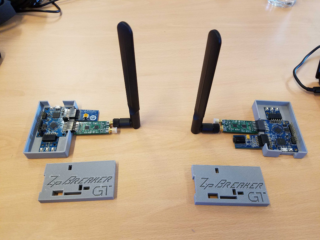Well, Edmund from Symbiotic EDA had asked me to build an FPGA radio core for him–just some simple demonstrator cores that could be used to help teach basic software defined radio principles to new and young engineers. The hardware I was given to use was an icebreaker FPGA board, and an SX1257 radio PMod. More specifically, I had two of each of these as shown in Fig. 1.

My thought was to use one of these as a transmitter, and the other as a receiver. Even better, I had a PMod MIC3 microphone from Digilent that I could use to capture audio for the transmitter, and a PMod AMP2 that I could use to drive a speaker. I’d used both of these before. They’re both easy to use and require little logic.

Put together, the entire system would look something like Fig. 2 below. An audio signal would enter the microphone, get encoded by the FPGA, and transmitted via the SX1257 PMod. On the other half, the reverse would be true: it would be received by the SX1257 PMod, demodulated by the FPGA design, amplified and then played out using a set of speakers.

Fig 2. Design components

I also thought I’d get a jump start on the problem by using AutoFPGA and a debugging bus. When I didn’t have an I2C controller suitable for the I2C to SPI bridge on the part, I reflected that I could bit-bang the configuration of the RF chip from an external CPU host.

My verification strategy was also very simple: I’d create four ports from within the RTL design of each modulation component, for both transmitter or receiver. These ports would output a stream of signal data from within the core to a place where I could capture that data with either a Wishbone scope or a histogram. This would allow me to verify that the data were sufficiently good before they ever got to the RF chip.

I then quickly drafted some awesomely grand designs: I built an AM transmitter core, an FM transmitter core, and even a 16QAM transmitter. I then built an AM and an FM receiver. (No, the 16QAM receiver isn’t done yet … which should come as no surprise to anyone familiar with the challenge.)

Of course, every good tragedy needs to start with a bit of hubris. In my case, I got sloppy. I didn’t build a simulation (initially). Why not? I wanted the design done fast. I had six days where I could work hand-in-hand with the engineers from Symbiotic EDA, and I couldn’t wait to see how this looked on a scope. What about bugs? I figured I could debug anything with my brand-new, wonderful histogram core together with my wishbone scope.

Care to hazard a guess at what was going to happen next?

Ok, now that you’ve ventured a guess, let’s see what actually happened.

It didn’t fit on the device

The first problem I had was that my initial design didn’t fit. Worse, it failed to fit in a way I wasn’t expecting: I’m used to working with designs that don’t have enough LUTs. If a DSP algorithm runs out of LUTs, I just lower the various bit-widths in the processing chain. I also know how to work around not having enough multiplies–by working at lower data rates and multiplexing the multiplies across the algorithm. You can also look to replace multiplies by shifts. No, in this case the design didn’t have enough block RAMs.

How much block RAM did I need?

I wanted 4kW (kilo-words) of 16-bit block RAM. The histogram implementation I had was going to double this into two areas of 4kW, so 8kW in total. That’s 256 kilobits, or 16 kilobytes.

Why did I want 256 kilobits? Because I could then split the histogram address space into a 6-bit X address and a 6-bit Y address. This would then allow me to generate a constellation diagram within the FPGA that would allow me to debug some of the higher order modulations–like my draft 16QAM transmitter. While I could use 5x5 bits, 6x6 would give me a clearer indication, in any 16QAM system, of what was working or not.

Sadly, those 16kB (kilobytes) of memory weren’t fitting on the device.

So I wandered over to Yosys’ iCE40 cell simulation library to understand just how much RAM I actually had available to me. NextPNR told me there were only 20 RAM cells on this chip. (There were actually 30, but I had NextPNR configured for the wrong chip at first.) I then went and found the library for the SiliconBlue RAM cell used by the iCE40 UP5K. With only a cursory glance, I discovered that this RAM required 11-bits of read (or write) address, and 16-bits of data. Perfect! That would make for 2kW of 16-bit RAM per block, so my design should fit in 8 blocks.

Why was yosys mapping my design to more than 20 blocks?

I decided to look deeper, and so I added a yosys command to output the synthesized netlist in Verilog form. Much to my surprise, it was only ever using four bits of this RAM at any given time.

Huh?

With some help from mwk, I learned that my cursory examination of the SB_RAM40_4K block was too cursory. The SB_RAM40_4K block only offered four kilobits of RAM. This ram had several configurations. It could be configured into 256 words of 16-bits each, requiring the 16-bit data width. It could also be configured into 2048 words of 2-bits each, requiring the 11-bit address width. Each of those configurations used exactly four kilobits of memory, and they were mutually exclusive. There was no configuration that used both 11 address bits and 16-data bits.

Apparently, this is common among FPGA architectures: to have a block of RAM that has multiple data and address width configurations.

Worse, my histogram implementation had two read ports. Since the iCE40 doesn’t have RAMs with dual read ports, Yosys was doubling my RAM usage to create two read ports. Each RAM was connected to the same write port, so each RAM would have the same contents, I could just read them from different places within my design.

Ok, I can deal with that. How hard can it be to adjust a design so that it shares a single read port between two pieces of logic? Just a couple changes should be sufficient:

I set the Wishbone stall signal, so that on any internal data read/update request within the histogram logic, the data request would get priority.

This shouldn’t slow down the Wishbone bus at all: the debugging core I was using was the hexbus we’d built together on this blog. It’s slow, but low logic. Moreover, the audio samples weren’t likely to generate constant valid signals into the histogram, so this should at most stall the bus by a single clock cycle.
I then added a new pipeline stage to the histogram’s to the processing chain–one where I calculated the memory address. While this didn’t seem to adjust the area much at all, I judged it to be a good addition. In my beginner’s tutorial, I discuss several rules of block RAM usage, one of which is that the address should always be registered. This change registered that address.

Just so you can understand how simple this change was, compare the two waveforms shown in Fig. 3 below.

Fig 3. Design waveform before and after the change
Before	With Changes

Here you can see how the stall line becomes the equivalent of the i_ce line, and how there’s now a new read_addr register multiplexing the two read requests together. You can also see how the data takes another clock before it can become valid.

Other changes

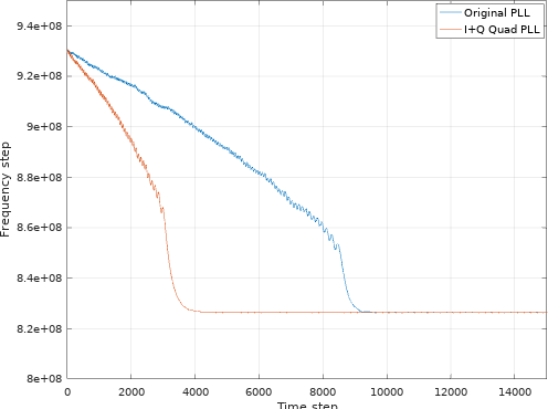
I did need to make some other changes as well. One in particular was needed for the AM demodulator. For this project, I needed an quadrature (complex I+Q) PLL, and the one we built together was only a single wire PLL.

This was easily adjusted for quadrature, and the resulting (simulated) performance appeared to be twice as good as the similar, single channel PLL implementation for the same PLL gain.

Fig 4. Comparing the original PLL with the I+Q Quadrature PLL

I’m going to try to remember to come back to this to make it an article in its own right–since the change was easy to do, and since I think it’d make an awesome blog article.

What happened?

Well, the updated design didn’t work. (Surprise!) Perhaps you figured out that this was going to happen from the setup above.

The first curious problem was that I was often not getting any data at all into the histogram. It would read all zeros.

This suggested that the i_ce signal was never getting set. We’ll look at what happened there in a moment.
When I did get a histogram result, it just looked like junk.

Was it just that the microphone was returning junk in the first place? That didn’t make sense, since I’d used the microphone SPI core before.
Often, the histogram might read like it was all large values. For example, when taking a histogram of 16k samples, adding all the elements together might result in over a million counts.

Ok, now that’s a clear bug.

What might the problem be?

As it turns out, there were several.

The first problem was associated with how I generated the sampling signal for the microphone. As is common with designs such as this, the signal processing chain can use the “global CE” strategy for pipeline signaling. Key to this strategy is to set the time when a new sample would be generated. For this I used a straight fractional clock divider.

        always @(posedge i_clk)
        if (!i_audio_en)
                { mic_ce, mic_ce_counter } <= 0;
        else
                { mic_ce, mic_ce_counter } <= mic_ce_counter + MIC_STEP;

Perhaps you may recall discussing this earlier? Or again when we discussed the units of phase in the NCO article?

The entire downsample rate was governed by a simple equation,

	localparam MIC_STEP = CLOCK_RATE_HZ * (1<<32) / AUDIO_SAMPLE_RATE;

Well, no, that didn’t work right. Worse, it doesn’t pass the smell test. (Remember studying units in science?) In this case, as the AUDIO_SAMPLE_RATE increases, the step size should increase–not decrease.

Let’s try that again.

	localparam MIC_STEP = AUDIO_SAMPLE_RATE * (1<<32) / CLOCK_RATE_HZ;

(This actually took me hours to find, since I was looking all over in the wrong places, but that’s another story.)

This change made things better, but they still weren’t quite right. Using this formula, the histogram would never count any samples coming into it: mic_ce was staying low. Indeed, if you dug into the design, mic_ce_counter was set to zero and never updated.

If you haven’t figured it yet, the hidden issue here is that all Verilog integers are 32-bits in size by default. In a 32-bit word, 1<<32 truncates to zero. This was not the desired effect I wanted.

One way around this is to use floating point values, and then to round the results to fixed point. We’ll also insist that 1<<32 be replaced with something that won’t overflow, 4.0 * (1<<30) for example.

	localparam [31:0] MIC_STEP = 4.0 * (1<<30) * AUDIO_SAMPLE_RATE
			* 1.0 / CLOCK_RATE_HZ;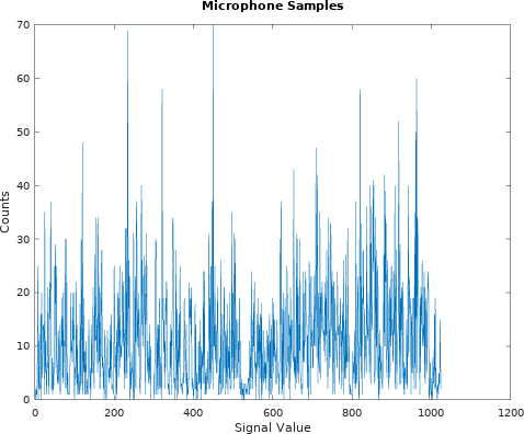

Fig 5. The histogram didn't look right

Now I could see samples coming from the histogram, as shown in Fig. 5.

Well, I suppose that’s better than all zeros. Only, it’s still not what I was expecting at all.

Were the incoming samples from the microphone really all that bad? Was I over driving the microphone? Sure, there was a lot of talking in a busy room, but I could still hear myself whisper.

After desk checking my design again for the umpteenth time looking for a bug, I decided to return to SymbiYosys and formally verify my changes to my histogram core.

What were the changes? Well, the biggest change was replacing the o_wb_stall signal,

	always @(*)
		o_wb_stall = 1'b0;

with a signal that would only accept an request if the i_ce signal, indicating a new incoming sample, was low.

	always @(*)
		o_wb_stall = i_ce;

I also replaced the read address to memory with a register that would select between one of two read addresses–either the one read from the bus, or the one to be written to in order to reflect the new data.

	always @(posedge i_clk)
	if (o_wb_stall)
		// Read a count to update it with a new sample
		read_addr <= { activemem, i_sample };
	else
		// Bus read
		read_addr <= { !activemem, i_wb_addr };

The one block RAM read would then read from this new address one clock later.

	always @(posedge i_clk)
		memval <= mem[read_addr];

The outgoing data was also adjusted. Instead of returning the value from the memory straight to the bus,

	always @(posedge i_clk)
	begin
		o_wb_data = 0;
		o_wb_data[ACCW-1:0] = mem[{ !activemem, i_wb_addr }];
	end

I would now return this intermediate value.

	always @(posedge i_clk)
	begin
		o_wb_data = 0;
		o_wb_data[ACCW-1:0] = memval;
	end

Looking through these changes, I didn’t see any problems. They all looked good to me. So, as I mentioned before, in a moment of frustration I turned to formal methods.

I also added my Wishbone property file to the formal proof. Sure, the Wishbone interaction was simple enough that I should’ve been able to verify it by eye, but I still couldn’t find the bug and it made sense to check all possibilities, and this was an easy one to check.

Once the properties were in place, I found the following in a matter of seconds.

	always @(posedge i_clk)
		o_wb_ack <= !reset && i_wb_stb;

This says that we’ll acknowledge a request immediately on the clock following the request. Notice how the acknowledgment isn’t dependent upon the stall signal, o_wb_stall.

One of the basic rules of bus property files is that there should never be any acknowledgments without prior requests. In this case, the formal tool held i_ce && i_wb_stb high long enough to get an o_wb_ack–even without i_wb_stb && !o_wb_stall ever having been true.

Staring at this some more, I realized that it would also take two clock cycles for any read, so I adjusted this ACK line for a two cycle read.

	initial { o_wb_ack, pre_ack } = 0;
	always @(posedge i_clk)
		pre_ack <= !i_reset && i_wb_stb && !o_wb_stall;
	always @(posedge i_clk)
		o_wb_ack <= !reset && i_wb_cyc && pre_ack;

Now the acknowledgment would match Fig. 3 above!

I was so excited! I’d now found my bug–after midnight, after I’d left the lab, etc. I was very excited to go to the lab the next day to check out how things had changed. Indeed, I was so excited about finding this bug that I started writing this article to share what had happened.

The good news is that, once I got to the lab, I was now getting different histograms.

Fig 6. First fix, but still not right

The bad news was that they still didn’t look right. Fig. 6 shows one of the traces I received after making the fix above.

At this point I finally bit the bullet and built a proper simulation of the design. In my simulation, I would feed a swept tone into the emulated microphone, and watch how the design responded. More specifically, I’d request a histogram, and then look at the trace of what was happening.

Sure enough, the simulation trace showed the problem: The acknowledgment was set one clock before the data was ready.

Did you catch that in the logic above? There was …

One clock to accept the bus request and set the address
One clock to read from memory (and set the acknowledgment), and
A third clock to return the results to the bus.

The third clock was simply added in because I didn’t quite think through what was going on. It would’ve helped if I had drawn out a design waveform, similar to Fig. 3 above, but, No, I didn’t do that until I started writing this article. Here was the block at fault.

	always @(posedge i_clk)
	begin
		o_wb_data = 0;
		o_wb_data[ACCW-1:0] = memval;
	end

One simple change fixed this bug.

	always @(*)	// <<---- The change
	begin
		o_wb_data = 0;
		o_wb_data[ACCW-1:0] = memval;
	end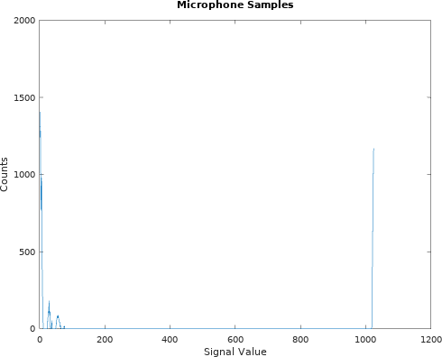

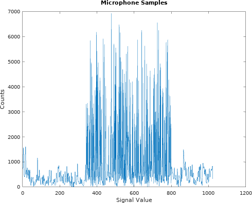
Fig 7. Histogram, now fixed

Once I made this change, the histogram started looking more reasonable. Fig. 7 on the right shows an example of the new histogram output. Indeed, this was very much what I was expecting.

Notice that all of the data are centered around either zero or the maximum value (i.e. -1, or in this case 10'h3ff). This would be indicative of an idle channel, where the microphone isn’t overloaded.

Perfect!

What about the fact that I was recording millions of counts from a 16k count histogram? That was now fixed. What was happening was that the data being sent to the core was routinely the most common value, causing the histogram to stall on a bus read, but then return the histogram point for that most common value rather than the point requested from the bus.

Shouldn’t this have been caught using formal methods? Indeed, it should have been. Then why didn’t my formal properties catch this?

Because I had used a cover() statement to capture the property that the right value would be returned from the bus, and not an assert() statement.

	cover property (@(posedge clk)
		// A read request, for our formally tracked value
		i_wb_stb && !o_wb_stall
			&& (i_wb_addr == f_addr[AW-1:0]) && activemem
			&& f_addr[AW] == !activemem
		//
		// The valid address cycle
		##1 i_wb_cyc && pre_ack
		//
		// The returned data cycle
		##2 o_wb_ack && o_wb_data[ACCW-1:0] == f_mem_data
			&& f_mem_data == 0);

Yes, it was possible to return the right value to the bus, and so the cover() statement passed. Had I expressed this in the form of an assert() statement, SymbiYosys would’ve caught the bug.

Conclusion

So, what sorts of conclusions can we draw from this?

Even the “perfect” core might need to be adjusted to fit the hardware du jour.
Sloppiness, whether by not formally verifying these changes or not building a simulation to check my work earlier, slowed me down. It didn’t speed me up–in spite of my best intentions.
From the “Tau of Programming” and roughly quoted, “Though a piece of code be but four lines long, someday it will need to be maintained.”

The entire design is now posted, although I’ll be the first to say that only the AM and FM modulations work, and even then they only work in simulation. Chances are I would’ve made more progress if I’d immediately gone to formal verification and then simulation, rather than trying to jump straight to the hardware where debugging is just that much more difficult. For now, the design will wait again in its current unfinished/limbo state until I have some more time to play with it.