
Using a CORDIC to calculate sines and cosines in an FPGA
We’ve now presented two separate algorithms that can be used for calculating a sine wave: a very simple sinewave table lookup, and a more complicated quarter-wave table lookup method. Both of these approaches used only a minimum number of clocks, although their precision was somewhat limited.
Today, let’s look at how to implement a COordinate Rotation DIgital Computer (CORDIC) algorithm within an FPGA.
 |
If you’ve never worked with a
CORDIC
algorithm before, the algorithms are all
based around specific
rotation matrices
which we will explain first. These rotation matrices can be strung together
to accomplish many digital logic purposes. For today’s discussion, though,
we will be rotating a two-dimensional vector by a requested counter-clockwise
angle. Thus, the inputs will be x and y values, i_xval and i_yval,
together with a requested phase rotation, i_phase, whereas the outputs
will just be a rotated x and y value, o_xval and o_yval–as shown in
Fig 1.
The CORDIC rotation
But, just what is a CORDIC rotation? Well, since all of these algorithms are built around a CORDIC rotation, let’s start by answering that question. We’ll start with the concept of a simple two-dimensional rotation matrix, and then work from there to how that can be turned into a CORDIC rotation.
A simple two-dimensional rotation matrix is given by:
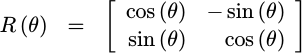 |
This rotation can be used to rotate a complex vector exp(j*phi) and turn it
into another one, exp(j*(phi+theta)), if the real value is the first value
in the given vector, and the would-be imaginary value the second (i.e. strip off
the j). Further, if the original vector is
simply the real number one, 1+j0, then we will have just created
sin(theta) and cos(theta) in this process.
This is what we are going to try to do: apply a rotation like this one.
We could apply this rotation using angles more suited for an FPGA,
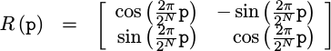 |
but this still leaves us with the problem that the sine and cosine aren’t easy to calculate, leaving this rotation difficult to accomplish.
 |
The
CORDIC
approach is to replace the cosine portion of this rotation matrix with a 1,
and the sine portion with a 2^-k.
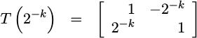 |
You can think of this as a series of complex rotation vectors,
indexed by k, such as those are shown in Fig 1. Notice from the figure
that these vectors are not on the unit circle, but rather just outside the
unit circle, and they get closer and closer to the unit circle the higher
k becomes.
In other words, T is approximately a
rotation matrix.
T is also something that is easy to calculate within an
FPGA.
It requires only adds, subtracts, and shifts.
 |
This can all be done with simple integer math–no multiplies or divides are required.
Of course, this transform is not a true rotation matrix. Instead, it is a scaled rotation matrix. To see this, first calculate the angles of the vectors in Fig 1 above:
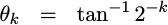 |
Then also calculate and normalize by their their lengths. The resulting
transform, T, is shown below:
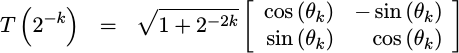 |
From here you can see that this is most definitely a rotation matrix with an amplitude increase associated with it.
Further, as you may have guessed from Fig 1 above, we can apply a similar rotation going in the opposite direction:
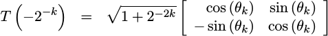 |
These two (nearly) rotation matrices form the basis of the CORDIC algorithm.
The basic idea behind the
CORDIC
algorithm is that we can string many of these
rotation matrices
together–either rotating by a positive theta_k or a
negative theta_k in each matrix. As an example, suppose you rotated
[1, 0] by +26.57 degrees (k=1), then by 14.03 degrees (k=2), then backwards
by 7.12 degrees (k=3). You would then
have a vector that has been rotated by 30.48 degrees. Other than
the slight amplitude increase, that means that your resulting vector now
approximates a thirty degree phasor–and you didn’t have to do anything that
significant to get there.
Further, the more of these rotation matrices you string together, the smaller the remaining rotation becomes, and hence the closer the result will come (in angular distance) to any desired rotation.
This is what we are going to try to build today.
Rotating into range
The first step in building this rotation, though, is to massage the problem
so that the rotation desired is less than 45 degrees. This comes from the
fact that the largest rotation the
CORDIC
rotation above can accomplish is a 45 degree rotation. Angles beyond
45 degrees just get smaller. Therefore, the
CORDIC
rotation requires an initial angular request, i_phase, to be less than 45
degrees. Our first problem, therefore is going to be rotating our incoming
vector so that any remaining rotation amount is 45 degrees or less.
As a preliminary step, we’ll start our algorithm off by expanding the two
input values from their initial width, IW, to a wider working width, WW.
Because the
CORDIC
algorithm will also increase the magnitude of the input, this process adds one
more bit on the left–to allow for a touch of width expansion. It also adds
a user selectable number of bits (captured as part of WW) to the right so as
to minimize any distortion’s caused by
truncation effects
within the rotation.
wire	signed [(WW-1):0]	e_xval, e_yval;
assign	e_xval = { {i_xval[(IW-1)]}, i_xval, {(WW-IW-1){1'b0}} };
assign	e_yval = { {i_yval[(IW-1)]}, i_yval, {(WW-IW-1){1'b0}} };
Further, we’re going to declare our intermediate values
to be an array of WW bits each for the intermediate xv and yv values,
and an array of phase width, PW, number of bits for the phase. Since the
CORDIC
operation takes place in stages, we’ll declare NSTAGES+1 of these
values–that will create variables to hold not only the input values,
but the outputs as well.
// Declare variables for all of the separate stages
reg	signed	[(WW-1):0]	xv	[0:(NSTAGES)];
reg	signed	[(WW-1):0]	yv	[0:(NSTAGES)];
reg		[(PW-1):0]	ph	[0:(NSTAGES)];
The beginner needs to understand that this is not the definition of a memory,
although it might look very similar to a block RAM definition. Rather, this
is a simplified definition of NSTAGES of values in flip-flops.
Declarations aside, that brings us to the actual logic of the pre-CORDIC section. The goal of this section is to rotate the input by some number of ninety-degree intervals until the remaining phase is between -45 and 45.
 |
Since this is a signal processing algorithm, the “global CE” pipeline
strategy
may make the most sense. We’ll also create logic for the traveling CE strategy
strategy
later. For now, remember that the global CE strategy requires that nothing
changes unless a CE line is true. Therefore, our transform begins by
checking the i_ce line.
always @(posedge i_clk)
if (i_ce)
Next, we’ll want to walk through the actual rotations.
 |
In order to get
everything into +/- 45 degrees, we’ll want to check not only which quadrant
our phase request is within, but also which 45 degree segment of that quadrant
the angle is in, as shown in Fig 3.
Hence, we’ll check the top three bits of i_phase, and apply a rotation
based upon them.
case(i_phase[(PW-1):(PW-3)])Each rotation opportunity will set xv[0], yv[0], and ph[0]. These are
the initial values of x, y, and the remaining phase to rotate through. The
options for xv[0] are +/- e_xval or +/- e_yval and likewise for yv[0].
Further, because these rotations are all by multiples of ninety degrees,
there’s no need to do any additions.
	3'b000: begin	// 0 .. 45, No change
		xv[0] <= e_xval;
		yv[0] <= e_yval;
		ph[0] <= i_phase;
		end
	3'b001: begin	// 45 .. 90
		xv[0] <= -e_yval;
		yv[0] <= e_xval;
		ph[0] <= i_phase - 18'h10000;
		end
	3'b010: begin	// 90 .. 135
		xv[0] <= -e_yval;
		yv[0] <= e_xval;
		ph[0] <= i_phase - 18'h10000;
		end
	3'b011: begin	// 135 .. 180
		xv[0] <= -e_xval;
		yv[0] <= -e_yval;
		ph[0] <= i_phase - 18'h20000;
		end
	3'b100: begin	// 180 .. 225
		xv[0] <= -e_xval;
		yv[0] <= -e_yval;
		ph[0] <= i_phase - 18'h20000;
		end
	3'b101: begin	// 225 .. 270
		xv[0] <= e_yval;
		yv[0] <= -e_xval;
		ph[0] <= i_phase - 18'h30000;
		end
	3'b110: begin	// 270 .. 315
		xv[0] <= e_yval;
		yv[0] <= -e_xval;
		ph[0] <= i_phase - 18'h30000;
		end
	3'b111: begin	// 315 .. 360, No change
		xv[0] <= e_xval;
		yv[0] <= e_yval;
		ph[0] <= i_phase;
		end
	endcase
Remember: we are rotating the xv and yv vector counter-clockwise, so
that the rotation remaining, ph, is less than +/- 45 degrees. Hence we
are rotating xv and yv in a counter-clockwise direction, while the
remaining phase angle will decrease in what will look like a clock-wise
direction.
This sets up the actual
CORDIC:
xv[0] and yv[0] now need to be rotated
through ph[0] remaining angular
units. We’ve also
guaranteed that |ph[0]| is less than or equal to 45 degrees.
Rotating to zero
The next step is to rotate the xv[0] and yv[0] values through the remaining
phase angle, ph[0]. To do this, we’re going to check whether or not the
remaining phase is negative or positive. If the phase is negative, we’ll
rotate by a positive cordic_angle[i]. If the remaining phase is positive,
we’ll rotate in the opposite direction but by the same amount.
Software programmers like to look at for and while loops in Verilog and
think of them like their for and while counterparts in software. HDL
loops, however, are nothing like software loops. Software loops repeat the
same instruction, one after another in time. HDL loops on the other hand
repeat the instruction in space on the chip by creating multiple copies of
the same logic, all of which will be executed in parallel.
This is one of those rare cases where a for loop makes sense in Verilog. The
CORDIC
algorithm repeats nearly the same logic NSTAGES times over. Hence, this
loop generates NSTAGES pieces of logic, each of which advances the
prior stage by one clock.
genvar	i;
generate for(i=0; i<NSTAGES; i=i+1) begin : CORDICops
Within this for loop, we’ll create several always blocks. Each block
first makes sure that nothing changes, except when the global CE signal, i_ce
is high.
always @(posedge i_clk)
// Reset logic can be placed here, but it isnt required
if (i_ce)
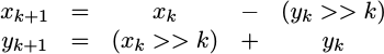
beginOnce these last preliminaries have been taken care of, we can finally apply the CORDIC rotation/transform. Note that we first check the sign of the remaining phase to know which direction to rotate, but otherwise the operations you see here should match the transform we discussed earlier.
		// You can check for cord[i] == 0 here if you would like
		if (ph[i][(PW-1)]) // Negative phase
		begin
			// If the phase is negative, rotate by the
			// CORDIC angle in a clockwise direction.
			xv[i+1] <= xv[i] + (yv[i]>>>(i+1));
			yv[i+1] <= yv[i] - (xv[i]>>>(i+1));
			ph[i+1] <= ph[i] + cordic_angle[i];

		end else begin
			// On the other hand, if the phase is
			// positive ... rotate in the
			// counter-clockwise direction
			xv[i+1] <= xv[i] - (yv[i]>>>(i+1));
			yv[i+1] <= yv[i] + (xv[i]>>>(i+1));
			ph[i+1] <= ph[i] - cordic_angle[i];

		end
	end
endgenerate
While this is the core of the
CORDIC
algorithm, now that we have put it together we are by no means done. We still
need to generate the CORDIC
angles, listed as array elements of cordic_angle above, any traveling
CE pipeline
logic,
drop any excess bits
we’ve accumulated,
and figure out what the gain of the algorithm is in case we wish to compensate
for it.
Using a core-generator in C++ to get the angles
One difficulty associated with building a “generic” CORDIC HDL core is that some of the components of the core cannot be generalized very easily. A good example of this problem is the VHDL CORDIC core found on OpenCores.
This open-cores core is built with a fixed precision. While the data width can ostensibly be adjusted, there are a fixed number of internal arc-tangent results, each created with a fixed width and a fixed value. (Well, that and you can’t simulate the core within Verilator because someone chose to write it within VHDL.) The only way to prevent this bit-width problem associated with a one-size fits all solution is to use a software program, sometimes called a core generator or coregen, to tailor the CORDIC to a specifically requested precision. This piece of software needs to calculate the phase rotation angles. We’ll also use the software to calculate the required number of stages, the number of input or output bits required, the number of phase bits, etc., etc.
Such a core generator will be our approach here. You can find the basic core generator here, within my cordic repository. For now, let’s discuss calculating the CORDIC angles.
Starting from above, the cordic angles are defined as
|
but in our normalized integer units of phase, the value we will want is going to be
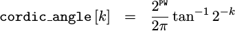 |
This value can easily be computed in C++ or any other higher level language for that matter. We’ll use C++ for this exercise.
We’ll need to calculate one angle for each of the CORDIC stages.
for(unsigned k=0; k<(unsigned)nstages; k++) {
	double		x, deg;
	unsigned	phase_value;
The angle is given by the arctangent of our rotation vector, 1+j2^-k.
x = atan2(1., pow(2,k));(Remember, atan2 accepts the y argument first. Hence our arguments of
x=2^k and y=1 represent an equivalent representation to our angle of
interest.)
We’ll keep track of the value of this angle in degrees as well as FPGA units,
deg = x * 180.0 / M_PI;For all other purposes, though, we’ll convert our angle to a normalized integer phase, value we can use in an FPGA algorithm,
	x *= (4.0 * (1ul<<(phase_bits-2))) / (M_PI * 2.0);
	phase_value = (unsigned)x;
We can then print this value to our resulting Verilog file.
	fprintf(fp, "\tassign\tcordic_angle[%2d] = %2d\'h%0*x; //%11.6f deg\n",
		k, phase_bits, (phase_bits+3)/4, phase_value,
		deg);
}
(I know this is the old-style C I/O — while I’ve used the C++ I/O, I’ve never really fallen in-love with it.)
After applying this calculation to a problem set with an 18-bit phase
requirement, the code above generated the following table,
assign	cordic_angle[ 0] = 18'h0_4b90; //  26.565051 deg
assign	cordic_angle[ 1] = 18'h0_27ec; //  14.036243 deg
assign	cordic_angle[ 2] = 18'h0_1444; //   7.125016 deg
assign	cordic_angle[ 3] = 18'h0_0a2c; //   3.576334 deg
assign	cordic_angle[ 4] = 18'h0_0517; //   1.789911 deg
assign	cordic_angle[ 5] = 18'h0_028b; //   0.895174 deg
assign	cordic_angle[ 6] = 18'h0_0145; //   0.447614 deg
assign	cordic_angle[ 7] = 18'h0_00a2; //   0.223811 deg
assign	cordic_angle[ 8] = 18'h0_0051; //   0.111906 deg
assign	cordic_angle[ 9] = 18'h0_0028; //   0.055953 deg
assign	cordic_angle[10] = 18'h0_0014; //   0.027976 deg
assign	cordic_angle[11] = 18'h0_000a; //   0.013988 deg
assign	cordic_angle[12] = 18'h0_0005; //   0.006994 deg
assign	cordic_angle[13] = 18'h0_0002; //   0.003497 deg
The number of stages and the number of bits in each stage can both be defined based upon arguments to the core generator program.
We still have several steps remaining. In particular, we need to set up the “traveling CE” pipeline strategy logic, round the final result, and discuss on how to deal with the amplitude distortion produced by the CORDIC algorithm.
Auxiliary Logic
I mentioned earlier that we could use the “traveling CE” pipeline strategy if desired. That strategy requires that for every strobe input, the output associated with that input also needs to have a high strobe output.
We’ll use our C++ code to build this as well, since in C++ we have control over when to place this logic into the code, as well as how much of this logic needs to be placed into our core.
To do this, we’ll teach the main core generator
program
to accept a -a option. We’ll then use this to create an auxiliary bit
to contain the “traveling CE” bit.
The actual logic required to implement this “traveling CE” is just a simple shift register:
always @(posedge i_clk)
	if (i_reset)
		ax <= {(NSTAGES+1){1'b0}};
	else if (i_ce)
		ax <= { ax[(NSTAGES-1):0], i_aux };

always @(posedge i_clk)
	o_aux <= ax[NSTAGES];
Were we to get rid of the reset, then all of this logic could fit within one shift register logic block on a 7-Series Xilinx FPGA. With the reset, this will require 1-FF per stage.
Placing this logic within the core generator makes certain that no matter
what logic takes place within the core, the output o_aux bit remains lined
up with the output data associated with any input data that had the i_aux
bit.
Dropping the last number of bits
When we get to the end, we’ll want to drop some bits. We discussed some time ago how to go about this via rounding. We also discussed several different types of rounding at that same time. Here, we follow the convergent rounding approach to drop any excess bits.
	// Round our result towards even
	wire	[(WW-1):0]	pre_xval, pre_yval;

	assign	pre_xval = xv[NSTAGES] + {{(OW){1'b0}},
				xv[NSTAGES][(WW-OW)],
				{(WW-OW-1){!xv[NSTAGES][WW-OW]}}};
	assign	pre_yval = yv[NSTAGES] + {{(OW){1'b0}},
				yv[NSTAGES][(WW-OW)],
				{(WW-OW-1){!yv[NSTAGES][WW-OW]}}};

	always @(posedge i_clk)
	begin
		o_xval <= pre_xval[(WW-1):(WW-OW)];
		o_yval <= pre_yval[(WW-1):(WW-OW)];
	end
That marks the end of our basic CORDIC algorithm. We still need to discuss what to do about the amplitude gain we’ve accumulated, so that will be next.
Dealing with Amplitude
As you’ll recall from the beginning of our discussion, the CORDIC algorithm has a gain associated with it. Our task here will be to calculate that gain. We’ll do this within our C++ generator program, since it has all the details and capability to do so.
Below is a copy of the C++ code used to calculate the cordic gain. It basically calculates the product of all of the gains of the various stages in our algorithm.
double	cordic_gain(int nstages, int phase_bits) {
	double	gain = 1.0;

	for(int k=0; k<nstages; k++) {
		double		dgain;

		dgain = 1.0 + pow(2.0,-2.*(k));
		dgain = sqrt(dgain);
		gain = gain * dgain;
	}

	return gain;
}
This, however, only tells us how much gain will be applied to our input. That
is, it quantifies our amplitude distortion. We’ll capture this with a
comment line added to the end of the list of cordic_angles.
// Gain is 1.646760Not all applications need gain compensation. Some can ignore the gain. In the case of those applications, the task is done.
Other applications use a
CORDIC
for calculating sines and cosines. These applications would nominally send
(1,0) into the algorithm as an input. For these applications, the way to
compensate for the gain is to send a different number as an input. Instead
of 1 (or really 2^n for an n-bit input), these algorithms will want
to send one divided by the gain into the algorithm. If we calculate the
right constant to replace the 1 with, then we still won’t need any
multiplies. To help you figure this out, the algorithm calculates
2^32/cordic_gain, and places this into the comments following the
calculation of the cordic_angles as well.
// You can annihilate this gain by multiplying by 32'h9b74edae
// and right shifting by 32 bits.
That allows you to pick the number of most-significant bits that you need, for the precision you want.
Other applications use the CORDIC to actually rotate the input vector. For these applications, the same 32-bit value can be used as an annihilator, post CORDIC application. If you multiply by this annihilator, and shift right, then the CORDIC gain will be removed.
Conclusions
Now that you’ve seen what goes into making a working CORDIC core, perhaps you are as amazed as I am at how many parts and pieces this simple sine and cosine wave generator has. We started out by discussing the rotation matrices used by the CORDIC algorithm. This is usually where most academic CORDIC development’s stop.
However, when you want to make a working CORDIC core, you have to go further. You need to rotate the original vector by some multiple of ninety degree angles until the remaining rotation angle is less than forty five degrees. Only then can you apply the CORDIC rotation. Doing so, though, requires the CORDIC angles, which we needed to calculate based upon the desired precision of the output. As a final step, we calculated both the CORDIC gain and it’s associated annihilator (inverse).
If only this were all that was required of a CORDIC core. It’s not. We still need to build a test bench for this core–so our work isn’t over yet. Before doing so, however, I think we’ll present the other basic type of CORDIC algorithm: the CORDIC arctan arctan, sometimes called the rectangular to polar conversion, before diving into the bench test.
If you are interested in further reading on the topic, Ray Andraka has written an excellent survey of CORDIC algorithms that you might find valuable.
O ye simple, understand wisdom: and, ye fools, be ye of an understanding heart. (Prov 8:5)